Repository of Reproducible Computations

Free Statistics

of Irreproducible Research!

Author's title

Author

*The author of this computation has been verified*

R Software Module

rwasp_edabi.wasp

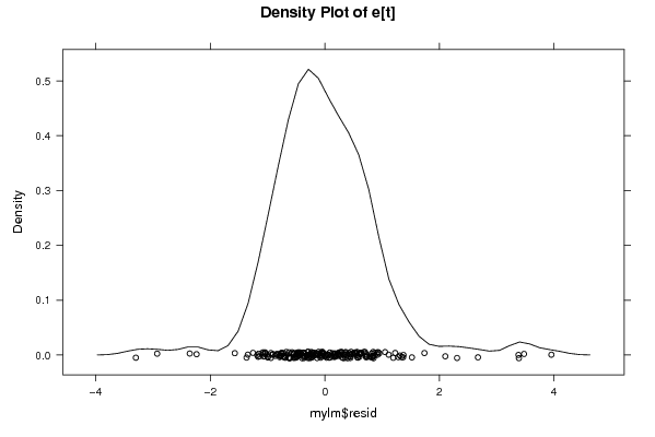
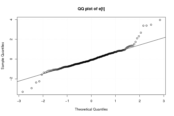
Title produced by software

Bivariate Explorative Data Analysis

Date of computation

Thu, 29 Oct 2009 11:44:27 -0600

Cite this page as follows

Statistical Computations at FreeStatistics.org, Office for Research Development and Education, URL https://freestatistics.org/blog/index.php?v=date/2009/Oct/29/t1256838336ld608leeficlgm7.htm/, Retrieved Sun, 28 Apr 2024 21:10:40 +0000

Statistical Computations at FreeStatistics.org, Office for Research Development and Education, URL https://freestatistics.org/blog/index.php?pk=52025, Retrieved Sun, 28 Apr 2024 21:10:40 +0000

QR Codes:

Paste this QR Code to cite your computation.

Original text written by user:

IsPrivate?

No (this computation is public)

User-defined keywords

Estimated Impact

154

Family? (F = Feedback message, R = changed R code, M = changed R Module, P = changed Parameters, D = changed Data)

-     [Trivariate Scatterplots] [SHW_WS5] [2009-10-29 16:26:54] [8b1aef4e7013bd33fbc2a5833375c5f5]
- RMPD    [Bivariate Explorative Data Analysis] [SHW_WS5] [2009-10-29 17:44:27] [f0f26816ac6124f58333f11f6c174000] [Current]
-  M D      [Bivariate Explorative Data Analysis] [ws 5] [2009-11-01 17:19:37] [b5908418e3090fddbd22f5f0f774653d] 
-  M        [Bivariate Explorative Data Analysis] [] [2009-11-04 11:57:05] [08fc5c07292c885b941f0cb515ce13f3] 
-  M D      [Bivariate Explorative Data Analysis] [] [2009-11-04 17:11:54] [44aba10e04b8829f2a97df951213e00a] 
-  M D      [Bivariate Explorative Data Analysis] [WS5(1)] [2009-11-04 17:11:54] [7d268329e554b8694908ba13e6e6f258] 
-    D        [Bivariate Explorative Data Analysis] [WS5(2)] [2009-11-04 17:41:47] [7d268329e554b8694908ba13e6e6f258] 
- RM D      [Bivariate Explorative Data Analysis] [Y=f(Z)] [2009-12-28 14:37:02] [2663058f2a5dda519058ac6b2228468f] 
-    D        [Bivariate Explorative Data Analysis] [X=f(Z)] [2009-12-28 14:49:17] [2663058f2a5dda519058ac6b2228468f] 
- RM D      [Bivariate Explorative Data Analysis] [X=f(Z)] [2009-12-28 14:41:24] [2663058f2a5dda519058ac6b2228468f] 
- RM D      [Bivariate Explorative Data Analysis] [model_3a] [2009-12-29 09:34:10] [2663058f2a5dda519058ac6b2228468f] 
- RM D      [Bivariate Explorative Data Analysis] [model_3b] [2009-12-29 09:39:08] [2663058f2a5dda519058ac6b2228468f] 
- RM D      [Bivariate Explorative Data Analysis] [model_3] [2009-12-29 09:45:53] [2663058f2a5dda519058ac6b2228468f] 

Feedback Forum

Post a new message

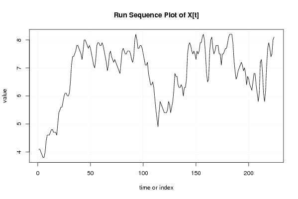
Dataseries X:

Download CSV

Histogram

Boxplots

4.1
4.1
4
3.9
3.8
3.8
4
4.4
4.6
4.6
4.6
4.7
4.8
4.8
4.7
4.7
4.7
4.6
5
5.4
5.5
5.6
5.6
5.8
6
6.1
6.1
6
6
6.1
6.5
7.1
7.4
7.4
7.5
7.6
7.8
7.8
7.7
7.6
7.5
7.3
7.6
8
8
7.9
7.8
7.7
7.8
7.7
7.5
7.3
7.1
7
7.3
7.8
7.9
7.9
7.8
7.8
7.9
7.8
7.6
7.4
7.2
6.9
7.1
7.5
7.6
7.4
7.3
7.2
7.3
7.2
7.1
7
6.9
6.8
7.2
7.6
7.7
7.6
7.5
7.5
7.6
7.6
7.6
7.5
7.3
7.2
7.4
8
8.2
8
7.7
7.7
7.8
7.8
7.7
7.5
7.3
7.1
7.1
7.2
6.8
6.6
6.4
6.4
6.5
6.3
5.9
5.5
5.2
4.9
5.4
5.8
5.7
5.6
5.5
5.4
5.4
5.4
5.5
5.8
5.7
5.4
5.6
5.8
6.2
6.8
6.7
6.7
6.4
6.3
6.3
6.4
6.3
6
6.3
6.3
6.6
7.5
7.8
7.9
7.8
7.6
7.5
7.6
7.5
7.3
7.6
7.5
7.6
7.9
7.9
8.1
8.2
8
7.5
6.8
6.5
6.6
7.6
8
8.1
7.7
7.5
7.6
7.8
7.8
7.8
7.5
7.5
7.1
7.5
7.5
7.6
7.7
7.7
7.9
8.1
8.2
8.2
8.2
7.9
7.3
6.9
6.6
6.7
6.9
7
7.1
7.2
7.1
6.9
7
6.8
6.4
6.7
6.6
6.4
6.3
6.2
6.5
6.8
6.8
6.4
6.1
5.8
6.1
7.2
7.3
6.9
6.1
5.8
6.2
7.1
7.7
7.9
7.7
7.4
7.5
8
8.1

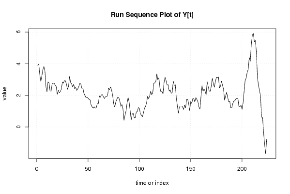
Dataseries Y:

Download CSV

Histogram

3.88
3.98
3.29
2.88
3.22
3.62
3.82
3.54
2.53
2.22
2.85
2.78
2.28
2.26
2.71
2.77
2.77
2.64
2.56
2.07
2.32
2.16
2.23
2.4
2.84
2.77
2.93
2.91
2.69
2.38
2.58
3.19
2.82
2.72
2.53
2.7
2.42
2.5
2.31
2.41
2.56
2.76
2.71
2.44
2.46
2.12
1.99
1.86
1.88
1.82
1.74
1.71
1.38
1.27
1.19
1.28
1.19
1.22
1.47
1.46
1.96
1.88
2.03
2.04
1.9
1.8
1.92
1.92
1.97
2.46
2.36
2.53
2.31
1.98
1.46
1.26
1.58
1.74
1.89
1.85
1.62
1.3
1.42
1.15
0.42
0.74
1.02
1.51
1.86
1.59
1.03
0.44
0.82
0.86
0.58
0.59
0.95
0.98
1.23
1.17
0.84
0.74
0.65
0.91
1.19
1.3
1.53
1.94
1.79
1.95
2.26
2.04
2.16
2.75
2.79
2.88
3.36
2.97
3.1
2.49
2.2
2.25
2.09
2.79
3.14
2.93
2.65
2.67
2.26
2.35
2.13
2.18
2.9
2.63
2.67
1.81
1.33
0.88
1.28
1.26
1.26
1.29
1.1
1.37
1.21
1.74
1.76
1.48
1.04
1.62
1.49
1.79
1.8
1.58
1.86
1.74
1.59
1.26
1.13
1.92
2.61
2.26
2.41
2.26
2.03
2.86
2.55
2.27
2.26
2.57
3.07
2.76
2.51
2.87
3.14
3.11
3.16
2.47
2.57
2.89
2.63
2.38
1.69
1.96
2.19
1.87
1.6
1.63
1.22
1.21
1.49
1.64
1.66
1.77
1.82
1.78
1.28
1.29
1.37
1.12
1.51
2.24
2.94
3.09
3.46
3.64
4.39
4.15
5.21
5.8
5.91
5.39
5.46
4.72
3.14
2.63
2.32
1.93
0.62
0.6
-0.37
-1.1
-1.68
-0.78

Summary of computational transaction
Raw Input	view raw input (R code)
Raw Output	view raw output of R engine
Computing time	4 seconds
R Server	'Sir Ronald Aylmer Fisher' @ 193.190.124.24

\begin{tabular}{lllllllll}
\hline
Summary of computational transaction \tabularnewline
Raw Input & view raw input (R code)  \tabularnewline
Raw Output & view raw output of R engine  \tabularnewline
Computing time & 4 seconds \tabularnewline
R Server & 'Sir Ronald Aylmer Fisher' @ 193.190.124.24 \tabularnewline
\hline
\end{tabular}
%Source: https://freestatistics.org/blog/index.php?pk=52025&T=0

[TABLE]
[ROW][C]Summary of computational transaction[/C][/ROW]
[ROW][C]Raw Input[/C][C]view raw input (R code) [/C][/ROW]
[ROW][C]Raw Output[/C][C]view raw output of R engine [/C][/ROW]
[ROW][C]Computing time[/C][C]4 seconds[/C][/ROW]
[ROW][C]R Server[/C][C]'Sir Ronald Aylmer Fisher' @ 193.190.124.24[/C][/ROW]
[/TABLE]
Source: https://freestatistics.org/blog/index.php?pk=52025&T=0

Globally Unique Identifier (entire table): ba.freestatistics.org/blog/index.php?pk=52025&T=0

As an alternative you can also use a QR Code:

The GUIDs for individual cells are displayed in the table below:

Summary of computational transaction
Raw Input	view raw input (R code)
Raw Output	view raw output of R engine
Computing time	4 seconds
R Server	'Sir Ronald Aylmer Fisher' @ 193.190.124.24

Model: Y[t] = c + b X[t] + e[t]
c	4.9502763299208
b	-0.416028181457045

\begin{tabular}{lllllllll}
\hline
Model: Y[t] = c + b X[t] + e[t] \tabularnewline
c & 4.9502763299208 \tabularnewline
b & -0.416028181457045 \tabularnewline
\hline
\end{tabular}
%Source: https://freestatistics.org/blog/index.php?pk=52025&T=1

[TABLE]
[ROW][C]Model: Y[t] = c + b X[t] + e[t][/C][/ROW]
[ROW][C]c[/C][C]4.9502763299208[/C][/ROW]
[ROW][C]b[/C][C]-0.416028181457045[/C][/ROW]
[/TABLE]
Source: https://freestatistics.org/blog/index.php?pk=52025&T=1

Globally Unique Identifier (entire table): ba.freestatistics.org/blog/index.php?pk=52025&T=1

As an alternative you can also use a QR Code:

The GUIDs for individual cells are displayed in the table below:

Model: Y[t] = c + b X[t] + e[t]
c	4.9502763299208
b	-0.416028181457045

Descriptive Statistics about e[t]
# observations	224
minimum	-3.30205087826444
Q1	-0.521763559920109
median	-0.0732706052843702
mean	8.00954354923666e-18
Q3	0.462644189980579
maximum	3.95512657656993

\begin{tabular}{lllllllll}
\hline
Descriptive Statistics about e[t] \tabularnewline
# observations & 224 \tabularnewline
minimum & -3.30205087826444 \tabularnewline
Q1 & -0.521763559920109 \tabularnewline
median & -0.0732706052843702 \tabularnewline
mean & 8.00954354923666e-18 \tabularnewline
Q3 & 0.462644189980579 \tabularnewline
maximum & 3.95512657656993 \tabularnewline
\hline
\end{tabular}
%Source: https://freestatistics.org/blog/index.php?pk=52025&T=2

[TABLE]
[ROW][C]Descriptive Statistics about e[t][/C][/ROW]
[ROW][C]# observations[/C][C]224[/C][/ROW]
[ROW][C]minimum[/C][C]-3.30205087826444[/C][/ROW]
[ROW][C]Q1[/C][C]-0.521763559920109[/C][/ROW]
[ROW][C]median[/C][C]-0.0732706052843702[/C][/ROW]
[ROW][C]mean[/C][C]8.00954354923666e-18[/C][/ROW]
[ROW][C]Q3[/C][C]0.462644189980579[/C][/ROW]
[ROW][C]maximum[/C][C]3.95512657656993[/C][/ROW]
[/TABLE]
Source: https://freestatistics.org/blog/index.php?pk=52025&T=2

Globally Unique Identifier (entire table): ba.freestatistics.org/blog/index.php?pk=52025&T=2

As an alternative you can also use a QR Code:

The GUIDs for individual cells are displayed in the table below:

Descriptive Statistics about e[t]
# observations	224
minimum	-3.30205087826444
Q1	-0.521763559920109
median	-0.0732706052843702
mean	8.00954354923666e-18
Q3	0.462644189980579
maximum	3.95512657656993

Figure 1

PNG link

Postscript link

PDF link

Figure 2

PNG link

Postscript link

PDF link

Figure 3

PNG link

Postscript link

PDF link

Figure 4

PNG link

Postscript link

PDF link

Figure 5

PNG link

Postscript link

PDF link

Figure 6

PNG link

Postscript link

PDF link

Figure 7

PNG link

Postscript link

PDF link

Figure 8

PNG link

Postscript link

PDF link

Parameters (Session):

par1 = 0 ; par2 = 36 ;

Parameters (R input):

par1 = 0 ; par2 = 36 ;

R code (references can be found in the software module):

par1 <- as.numeric(par1)
par2 <- as.numeric(par2)
x <- as.ts(x)
y <- as.ts(y)
mylm <- lm(y~x)
cbind(mylm$resid)
library(lattice)
bitmap(file='pic1.png')
plot(y,type='l',main='Run Sequence Plot of Y[t]',xlab='time or index',ylab='value')
grid()
dev.off()
bitmap(file='pic1a.png')
plot(x,type='l',main='Run Sequence Plot of X[t]',xlab='time or index',ylab='value')
grid()
dev.off()
bitmap(file='pic1b.png')
plot(x,y,main='Scatter Plot',xlab='X[t]',ylab='Y[t]')
grid()
dev.off()
bitmap(file='pic1c.png')
plot(mylm$resid,type='l',main='Run Sequence Plot of e[t]',xlab='time or index',ylab='value')
grid()
dev.off()
bitmap(file='pic2.png')
hist(mylm$resid,main='Histogram of e[t]')
dev.off()
bitmap(file='pic3.png')
if (par1 > 0)
{
densityplot(~mylm$resid,col='black',main=paste('Density Plot of e[t]   bw = ',par1),bw=par1)
} else {
densityplot(~mylm$resid,col='black',main='Density Plot of e[t]')
}
dev.off()
bitmap(file='pic4.png')
qqnorm(mylm$resid,main='QQ plot of e[t]')
qqline(mylm$resid)
grid()
dev.off()
if (par2 > 0)
{
bitmap(file='pic5.png')
acf(mylm$resid,lag.max=par2,main='Residual Autocorrelation Function')
grid()
dev.off()
}
summary(x)
load(file='createtable')
a<-table.start()
a<-table.row.start(a)
a<-table.element(a,'Model: Y[t] = c + b X[t] + e[t]',2,TRUE)
a<-table.row.end(a)
a<-table.row.start(a)
a<-table.element(a,'c',1,TRUE)
a<-table.element(a,mylm$coeff[[1]])
a<-table.row.end(a)
a<-table.row.start(a)
a<-table.element(a,'b',1,TRUE)
a<-table.element(a,mylm$coeff[[2]])
a<-table.row.end(a)
a<-table.end(a)
table.save(a,file='mytable.tab')
a<-table.start()
a<-table.row.start(a)
a<-table.element(a,'Descriptive Statistics about e[t]',2,TRUE)
a<-table.row.end(a)
a<-table.row.start(a)
a<-table.element(a,'# observations',header=TRUE)
a<-table.element(a,length(mylm$resid))
a<-table.row.end(a)
a<-table.row.start(a)
a<-table.element(a,'minimum',header=TRUE)
a<-table.element(a,min(mylm$resid))
a<-table.row.end(a)
a<-table.row.start(a)
a<-table.element(a,'Q1',header=TRUE)
a<-table.element(a,quantile(mylm$resid,0.25))
a<-table.row.end(a)
a<-table.row.start(a)
a<-table.element(a,'median',header=TRUE)
a<-table.element(a,median(mylm$resid))
a<-table.row.end(a)
a<-table.row.start(a)
a<-table.element(a,'mean',header=TRUE)
a<-table.element(a,mean(mylm$resid))
a<-table.row.end(a)
a<-table.row.start(a)
a<-table.element(a,'Q3',header=TRUE)
a<-table.element(a,quantile(mylm$resid,0.75))
a<-table.row.end(a)
a<-table.row.start(a)
a<-table.element(a,'maximum',header=TRUE)
a<-table.element(a,max(mylm$resid))
a<-table.row.end(a)
a<-table.end(a)
table.save(a,file='mytable.tab')

Free Statistics

Description of Statistical Computation

Tree of Dependent Computations

Dataset

Tables (Output of Computation)

Figures (Output of Computation)

Input Parameters & R Code