Free Statistics
of Irreproducible Research!
Description of Statistical Computation | |||||||||||||||||||||||||||||||||||||||||||||||||||||||||||||||||
|---|---|---|---|---|---|---|---|---|---|---|---|---|---|---|---|---|---|---|---|---|---|---|---|---|---|---|---|---|---|---|---|---|---|---|---|---|---|---|---|---|---|---|---|---|---|---|---|---|---|---|---|---|---|---|---|---|---|---|---|---|---|---|---|---|---|
| Author's title | |||||||||||||||||||||||||||||||||||||||||||||||||||||||||||||||||
| Author | *The author of this computation has been verified* | ||||||||||||||||||||||||||||||||||||||||||||||||||||||||||||||||
| R Software Module | rwasp_edabi.wasp | ||||||||||||||||||||||||||||||||||||||||||||||||||||||||||||||||
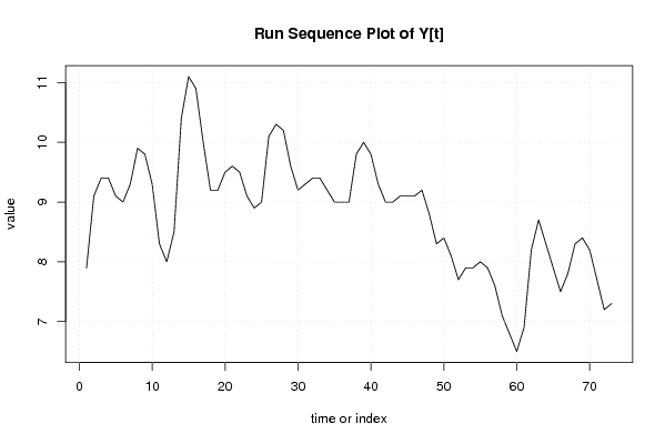
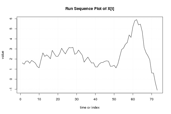
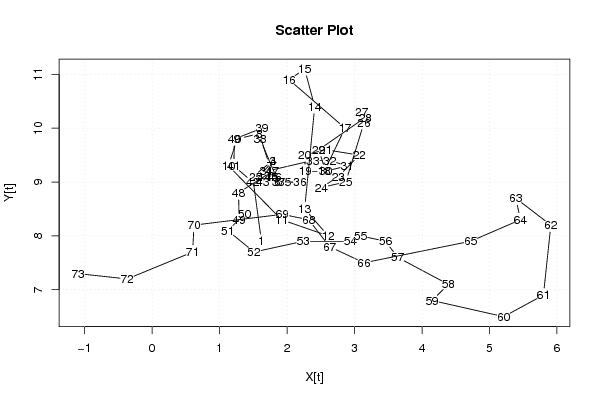
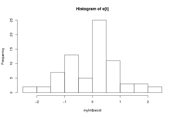
| Title produced by software | Bivariate Explorative Data Analysis | ||||||||||||||||||||||||||||||||||||||||||||||||||||||||||||||||
| Date of computation | Thu, 29 Oct 2009 09:21:11 -0600 | ||||||||||||||||||||||||||||||||||||||||||||||||||||||||||||||||
| Cite this page as follows | Statistical Computations at FreeStatistics.org, Office for Research Development and Education, URL https://freestatistics.org/blog/index.php?v=date/2009/Oct/29/t1256829744agwc8wrr45pw9sz.htm/, Retrieved Sun, 28 Apr 2024 21:04:58 +0000 | ||||||||||||||||||||||||||||||||||||||||||||||||||||||||||||||||
| Statistical Computations at FreeStatistics.org, Office for Research Development and Education, URL https://freestatistics.org/blog/index.php?pk=52009, Retrieved Sun, 28 Apr 2024 21:04:58 +0000 | |||||||||||||||||||||||||||||||||||||||||||||||||||||||||||||||||
| QR Codes: | |||||||||||||||||||||||||||||||||||||||||||||||||||||||||||||||||
|
| |||||||||||||||||||||||||||||||||||||||||||||||||||||||||||||||||
| Original text written by user: | |||||||||||||||||||||||||||||||||||||||||||||||||||||||||||||||||
| IsPrivate? | No (this computation is public) | ||||||||||||||||||||||||||||||||||||||||||||||||||||||||||||||||
| User-defined keywords | SHWWS5 Xt(werkloosheidsgraad vrouwen Z(inflatie) | ||||||||||||||||||||||||||||||||||||||||||||||||||||||||||||||||
| Estimated Impact | 186 | ||||||||||||||||||||||||||||||||||||||||||||||||||||||||||||||||
Tree of Dependent Computations | |||||||||||||||||||||||||||||||||||||||||||||||||||||||||||||||||
| Family? (F = Feedback message, R = changed R code, M = changed R Module, P = changed Parameters, D = changed Data) | |||||||||||||||||||||||||||||||||||||||||||||||||||||||||||||||||
| - [Bivariate Data Series] [Bivariate dataset] [2008-01-05 23:51:08] [74be16979710d4c4e7c6647856088456] - RMPD [Bivariate Explorative Data Analysis] [Bivariate EDA ana...] [2009-10-27 11:17:50] [4395c69e961f9a13a0559fd2f0a72538] - RMPD [Trivariate Scatterplots] [Trivariate Scatte...] [2009-10-29 14:00:50] [4395c69e961f9a13a0559fd2f0a72538] - RMP [Partial Correlation] [Partial Correlati...] [2009-10-29 14:05:54] [4395c69e961f9a13a0559fd2f0a72538] - RMPD [Bivariate Explorative Data Analysis] [Bivariate EDA Y[t] Z] [2009-10-29 14:14:40] [4395c69e961f9a13a0559fd2f0a72538] - D [Bivariate Explorative Data Analysis] [Bivariate EDA Y[t...] [2009-10-29 15:03:23] [4395c69e961f9a13a0559fd2f0a72538] - D [Bivariate Explorative Data Analysis] [Bivariate EDA X[t...] [2009-10-29 15:21:11] [d1081bd6cdf1fed9ed45c42dbd523bf1] [Current] - D [Bivariate Explorative Data Analysis] [Bivariate EDA e[t...] [2009-10-29 15:36:56] [4395c69e961f9a13a0559fd2f0a72538] - M D [Bivariate Explorative Data Analysis] [Paper Bivariate E...] [2009-12-17 15:39:37] [4395c69e961f9a13a0559fd2f0a72538] - M D [Bivariate Explorative Data Analysis] [Bivariate EDA X[t...] [2009-12-17 15:23:33] [4395c69e961f9a13a0559fd2f0a72538] | |||||||||||||||||||||||||||||||||||||||||||||||||||||||||||||||||
| Feedback Forum | |||||||||||||||||||||||||||||||||||||||||||||||||||||||||||||||||
Post a new message | |||||||||||||||||||||||||||||||||||||||||||||||||||||||||||||||||
Dataset | |||||||||||||||||||||||||||||||||||||||||||||||||||||||||||||||||
| Dataseries X: | |||||||||||||||||||||||||||||||||||||||||||||||||||||||||||||||||
1.62 1.49 1.79 1.8 1.58 1.86 1.74 1.59 1.26 1.13 1.92 2.61 2.26 2.41 2.26 2.03 2.86 2.55 2.27 2.26 2.57 3.07 2.76 2.51 2.87 3.14 3.11 3.16 2.47 2.57 2.89 2.63 2.38 1.69 1.96 2.19 1.87 1.6 1.63 1.22 1.21 1.49 1.64 1.66 1.77 1.82 1.78 1.28 1.29 1.37 1.12 1.51 2.24 2.94 3.09 3.46 3.64 4.39 4.15 5.21 5.8 5.91 5.39 5.46 4.72 3.14 2.63 2.32 1.93 0.62 0.6 -0.37 -1.1 | |||||||||||||||||||||||||||||||||||||||||||||||||||||||||||||||||
| Dataseries Y: | |||||||||||||||||||||||||||||||||||||||||||||||||||||||||||||||||
7.9 9.1 9.4 9.4 9.1 9 9.3 9.9 9.8 9.3 8.3 8 8.5 10.4 11.1 10.9 10 9.2 9.2 9.5 9.6 9.5 9.1 8.9 9 10.1 10.3 10.2 9.6 9.2 9.3 9.4 9.4 9.2 9 9 9 9.8 10 9.8 9.3 9 9 9.1 9.1 9.1 9.2 8.8 8.3 8.4 8.1 7.7 7.9 7.9 8 7.9 7.6 7.1 6.8 6.5 6.9 8.2 8.7 8.3 7.9 7.5 7.8 8.3 8.4 8.2 7.7 7.2 7.3 | |||||||||||||||||||||||||||||||||||||||||||||||||||||||||||||||||
Tables (Output of Computation) | |||||||||||||||||||||||||||||||||||||||||||||||||||||||||||||||||
| |||||||||||||||||||||||||||||||||||||||||||||||||||||||||||||||||
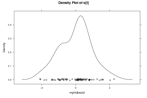
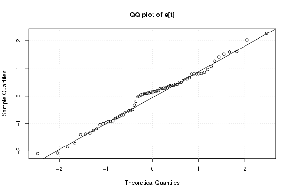
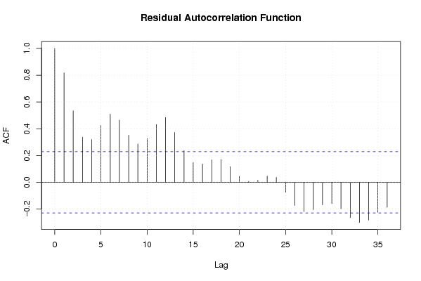
Figures (Output of Computation) | |||||||||||||||||||||||||||||||||||||||||||||||||||||||||||||||||
Input Parameters & R Code | |||||||||||||||||||||||||||||||||||||||||||||||||||||||||||||||||
| Parameters (Session): | |||||||||||||||||||||||||||||||||||||||||||||||||||||||||||||||||
| par1 = 0 ; par2 = 36 ; | |||||||||||||||||||||||||||||||||||||||||||||||||||||||||||||||||
| Parameters (R input): | |||||||||||||||||||||||||||||||||||||||||||||||||||||||||||||||||
| par1 = 0 ; par2 = 36 ; | |||||||||||||||||||||||||||||||||||||||||||||||||||||||||||||||||
| R code (references can be found in the software module): | |||||||||||||||||||||||||||||||||||||||||||||||||||||||||||||||||
par1 <- as.numeric(par1) | |||||||||||||||||||||||||||||||||||||||||||||||||||||||||||||||||