Free Statistics
of Irreproducible Research!
Description of Statistical Computation | |||||||||||||||||||||
|---|---|---|---|---|---|---|---|---|---|---|---|---|---|---|---|---|---|---|---|---|---|
| Author's title | |||||||||||||||||||||
| Author | *The author of this computation has been verified* | ||||||||||||||||||||
| R Software Module | rwasp_cloud.wasp | ||||||||||||||||||||
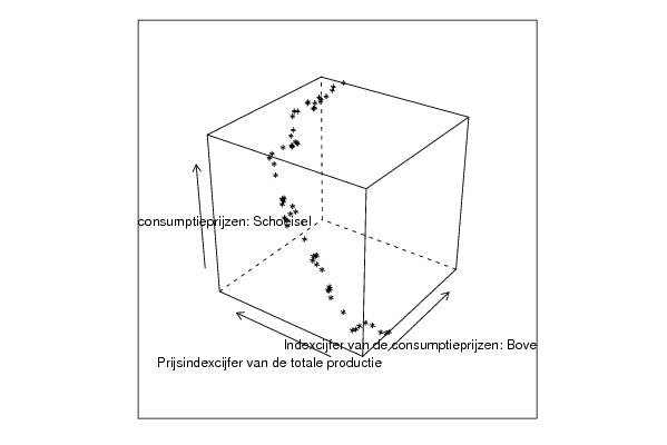
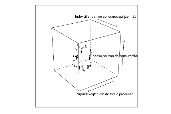
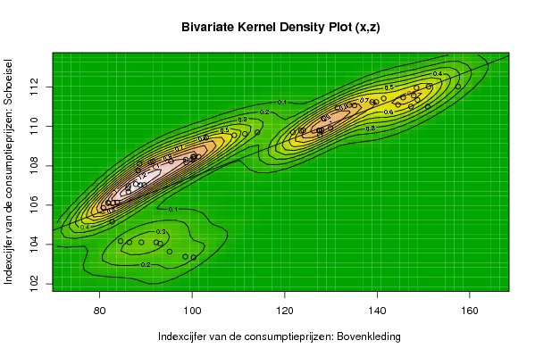
| Title produced by software | Trivariate Scatterplots | ||||||||||||||||||||
| Date of computation | Wed, 28 Oct 2009 16:35:45 -0600 | ||||||||||||||||||||
| Cite this page as follows | Statistical Computations at FreeStatistics.org, Office for Research Development and Education, URL https://freestatistics.org/blog/index.php?v=date/2009/Oct/28/t125676938147ljhh6vx4y49zg.htm/, Retrieved Mon, 06 May 2024 06:43:31 +0000 | ||||||||||||||||||||
| Statistical Computations at FreeStatistics.org, Office for Research Development and Education, URL https://freestatistics.org/blog/index.php?pk=51889, Retrieved Mon, 06 May 2024 06:43:31 +0000 | |||||||||||||||||||||
| QR Codes: | |||||||||||||||||||||
|
| |||||||||||||||||||||
| Original text written by user: | |||||||||||||||||||||
| IsPrivate? | No (this computation is public) | ||||||||||||||||||||
| User-defined keywords | |||||||||||||||||||||
| Estimated Impact | 118 | ||||||||||||||||||||
Tree of Dependent Computations | |||||||||||||||||||||
| Family? (F = Feedback message, R = changed R code, M = changed R Module, P = changed Parameters, D = changed Data) | |||||||||||||||||||||
| - [Trivariate Scatterplots] [WS 5 1] [2009-10-28 22:35:45] [2e4ef2c1b76db9b31c0a03b96e94ad77] [Current] - MPD [Trivariate Scatterplots] [DSHW-WS5-Trivaria...] [2009-11-03 17:42:05] [f15cfb7053d35072d573abca87df96a0] - RMPD [Bivariate Explorative Data Analysis] [DSHW-WS5-Bivariat...] [2009-11-03 18:01:01] [f15cfb7053d35072d573abca87df96a0] - RMPD [Kendall tau Correlation Matrix] [Kendell Tau corre...] [2009-11-07 15:38:04] [d31db4f83c6a129f6d3e47077769e868] - RMPD [Bivariate Explorative Data Analysis] [DSHW-WS5-NewBivar...] [2009-11-03 18:35:20] [f15cfb7053d35072d573abca87df96a0] | |||||||||||||||||||||
| Feedback Forum | |||||||||||||||||||||
Post a new message | |||||||||||||||||||||
Dataset | |||||||||||||||||||||
| Dataseries X: | |||||||||||||||||||||
100,30 98,50 95,10 93,10 92,20 89,00 86,40 84,50 82,70 80,80 81,80 81,80 82,90 83,80 86,20 86,10 86,20 88,80 89,60 87,80 88,30 88,60 91,00 91,50 95,40 98,70 99,90 98,60 100,30 100,20 100,40 101,40 103,00 109,10 111,40 114,10 121,80 127,60 129,90 128,00 123,50 124,00 127,40 127,60 128,40 131,40 135,10 134,00 144,50 147,30 150,90 148,70 141,40 138,90 139,80 145,60 147,90 148,50 151,10 157,50 | |||||||||||||||||||||
| Dataseries Y: | |||||||||||||||||||||
103,63 103,64 103,66 103,77 103,88 103,91 103,91 103,92 104,05 104,23 104,30 104,31 104,31 104,34 104,55 104,65 104,73 104,75 104,75 104,76 104,94 105,29 105,38 105,43 105,43 105,42 105,52 105,69 105,72 105,74 105,74 105,74 105,95 106,17 106,34 106,37 106,37 106,36 106,44 106,29 106,23 106,23 106,23 106,23 106,34 106,44 106,44 106,48 106,50 106,57 106,40 106,37 106,25 106,21 106,21 106,24 106,19 106,08 106,13 106,09 | |||||||||||||||||||||
| Dataseries Z: | |||||||||||||||||||||
103,34 103,38 103,64 104,04 104,11 104,11 104,11 104,17 105,16 105,86 106,11 106,11 106,11 106,13 106,67 106,85 106,97 107,02 107,02 107,07 107,76 108,10 108,18 108,22 108,22 108,17 108,31 108,31 108,36 108,46 108,46 108,46 109,43 109,55 109,62 109,70 109,70 109,56 109,92 109,81 109,78 109,80 109,80 109,79 110,40 110,95 111,07 111,09 111,10 111,01 111,01 111,35 111,42 111,24 111,24 111,47 111,57 111,96 112,02 112,02 | |||||||||||||||||||||
Tables (Output of Computation) | |||||||||||||||||||||
| |||||||||||||||||||||
Figures (Output of Computation) | |||||||||||||||||||||
Input Parameters & R Code | |||||||||||||||||||||
| Parameters (Session): | |||||||||||||||||||||
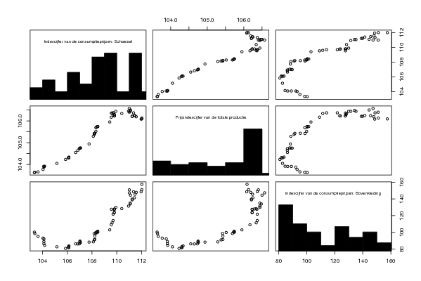
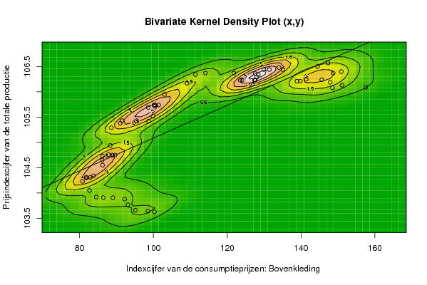
| par1 = 50 ; par2 = 50 ; par3 = Y ; par4 = Y ; par5 = Indexcijfer van de consumptieprijzen: Bovenkleding ; par6 = Prijsindexcijfer van de totale productie ; par7 = Indexcijfer van de consumptieprijzen: Schoeisel ; | |||||||||||||||||||||
| Parameters (R input): | |||||||||||||||||||||
| par1 = 50 ; par2 = 50 ; par3 = Y ; par4 = Y ; par5 = Indexcijfer van de consumptieprijzen: Bovenkleding ; par6 = Prijsindexcijfer van de totale productie ; par7 = Indexcijfer van de consumptieprijzen: Schoeisel ; | |||||||||||||||||||||
| R code (references can be found in the software module): | |||||||||||||||||||||
x <- array(x,dim=c(length(x),1)) | |||||||||||||||||||||