Free Statistics
of Irreproducible Research!
Description of Statistical Computation | |||||||||||||||||||||||||||||||||||||||||||||||||||||||||||||||||
|---|---|---|---|---|---|---|---|---|---|---|---|---|---|---|---|---|---|---|---|---|---|---|---|---|---|---|---|---|---|---|---|---|---|---|---|---|---|---|---|---|---|---|---|---|---|---|---|---|---|---|---|---|---|---|---|---|---|---|---|---|---|---|---|---|---|
| Author's title | |||||||||||||||||||||||||||||||||||||||||||||||||||||||||||||||||
| Author | *The author of this computation has been verified* | ||||||||||||||||||||||||||||||||||||||||||||||||||||||||||||||||
| R Software Module | rwasp_edabi.wasp | ||||||||||||||||||||||||||||||||||||||||||||||||||||||||||||||||
| Title produced by software | Bivariate Explorative Data Analysis | ||||||||||||||||||||||||||||||||||||||||||||||||||||||||||||||||
| Date of computation | Wed, 28 Oct 2009 12:28:17 -0600 | ||||||||||||||||||||||||||||||||||||||||||||||||||||||||||||||||
| Cite this page as follows | Statistical Computations at FreeStatistics.org, Office for Research Development and Education, URL https://freestatistics.org/blog/index.php?v=date/2009/Oct/28/t1256754599n9u20rl2k71i7ux.htm/, Retrieved Mon, 06 May 2024 04:35:47 +0000 | ||||||||||||||||||||||||||||||||||||||||||||||||||||||||||||||||
| Statistical Computations at FreeStatistics.org, Office for Research Development and Education, URL https://freestatistics.org/blog/index.php?pk=51707, Retrieved Mon, 06 May 2024 04:35:47 +0000 | |||||||||||||||||||||||||||||||||||||||||||||||||||||||||||||||||
| QR Codes: | |||||||||||||||||||||||||||||||||||||||||||||||||||||||||||||||||
|
| |||||||||||||||||||||||||||||||||||||||||||||||||||||||||||||||||
| Original text written by user: | |||||||||||||||||||||||||||||||||||||||||||||||||||||||||||||||||
| IsPrivate? | No (this computation is public) | ||||||||||||||||||||||||||||||||||||||||||||||||||||||||||||||||
| User-defined keywords | part 2 model 1 bivariate eda | ||||||||||||||||||||||||||||||||||||||||||||||||||||||||||||||||
| Estimated Impact | 118 | ||||||||||||||||||||||||||||||||||||||||||||||||||||||||||||||||
Tree of Dependent Computations | |||||||||||||||||||||||||||||||||||||||||||||||||||||||||||||||||
| Family? (F = Feedback message, R = changed R code, M = changed R Module, P = changed Parameters, D = changed Data) | |||||||||||||||||||||||||||||||||||||||||||||||||||||||||||||||||
| - [Bivariate Data Series] [Bivariate dataset] [2008-01-05 23:51:08] [74be16979710d4c4e7c6647856088456] - PD [Bivariate Data Series] [part 2 model 1] [2009-10-28 18:19:40] [616e2df490b611f6cb7080068870ecbd] - RMP [Bivariate Explorative Data Analysis] [part 2 model 1 bi...] [2009-10-28 18:28:17] [88e98f4c87ea17c4967db8279bda8533] [Current] - D [Bivariate Explorative Data Analysis] [part2 model 2 Biv...] [2009-10-28 18:56:15] [616e2df490b611f6cb7080068870ecbd] - D [Bivariate Explorative Data Analysis] [part 2 model 3 bi...] [2009-10-28 19:22:48] [616e2df490b611f6cb7080068870ecbd] - RMPD [Kendall tau Rank Correlation] [ws4 part 3] [2009-10-28 19:54:27] [616e2df490b611f6cb7080068870ecbd] | |||||||||||||||||||||||||||||||||||||||||||||||||||||||||||||||||
| Feedback Forum | |||||||||||||||||||||||||||||||||||||||||||||||||||||||||||||||||
Post a new message | |||||||||||||||||||||||||||||||||||||||||||||||||||||||||||||||||
Dataset | |||||||||||||||||||||||||||||||||||||||||||||||||||||||||||||||||
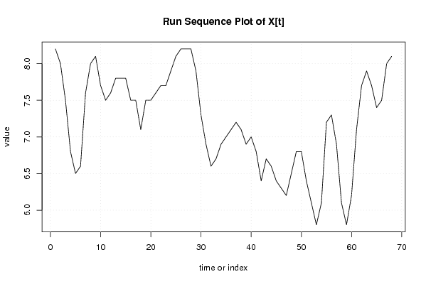
| Dataseries X: | |||||||||||||||||||||||||||||||||||||||||||||||||||||||||||||||||
8.2 8 7.5 6.8 6.5 6.6 7.6 8 8.1 7.7 7.5 7.6 7.8 7.8 7.8 7.5 7.5 7.1 7.5 7.5 7.6 7.7 7.7 7.9 8.1 8.2 8.2 8.2 7.9 7.3 6.9 6.6 6.7 6.9 7 7.1 7.2 7.1 6.9 7 6.8 6.4 6.7 6.6 6.4 6.3 6.2 6.5 6.8 6.8 6.4 6.1 5.8 6.1 7.2 7.3 6.9 6.1 5.8 6.2 7.1 7.7 7.9 7.7 7.4 7.5 8 8.1 | |||||||||||||||||||||||||||||||||||||||||||||||||||||||||||||||||
| Dataseries Y: | |||||||||||||||||||||||||||||||||||||||||||||||||||||||||||||||||
9.9 9.8 9.3 8.3 8.0 8.5 10.4 11.1 10.9 10.0 9.2 9.2 9.5 9.6 9.5 9.1 8.9 9.0 10.1 10.3 10.2 9.6 9.2 9.3 9.4 9.4 9.2 9.0 9.0 9.0 9.8 10.0 9.8 9.3 9.0 9.0 9.1 9.1 9.1 9.2 8.8 8.3 8.4 8.1 7.7 7.9 7.9 8.0 7.9 7.6 7.1 6.8 6.5 6.9 8.2 8.7 8.3 7.9 7.5 7.8 8.3 8.4 8.2 7.7 7.2 7.3 8.1 8.5 | |||||||||||||||||||||||||||||||||||||||||||||||||||||||||||||||||
Tables (Output of Computation) | |||||||||||||||||||||||||||||||||||||||||||||||||||||||||||||||||
| |||||||||||||||||||||||||||||||||||||||||||||||||||||||||||||||||
Figures (Output of Computation) | |||||||||||||||||||||||||||||||||||||||||||||||||||||||||||||||||
Input Parameters & R Code | |||||||||||||||||||||||||||||||||||||||||||||||||||||||||||||||||
| Parameters (Session): | |||||||||||||||||||||||||||||||||||||||||||||||||||||||||||||||||
| par1 = 0 ; par2 = 36 ; | |||||||||||||||||||||||||||||||||||||||||||||||||||||||||||||||||
| Parameters (R input): | |||||||||||||||||||||||||||||||||||||||||||||||||||||||||||||||||
| par1 = 0 ; par2 = 36 ; | |||||||||||||||||||||||||||||||||||||||||||||||||||||||||||||||||
| R code (references can be found in the software module): | |||||||||||||||||||||||||||||||||||||||||||||||||||||||||||||||||
par1 <- as.numeric(par1) | |||||||||||||||||||||||||||||||||||||||||||||||||||||||||||||||||