Free Statistics
of Irreproducible Research!
Description of Statistical Computation | |||||||||||||||||||||||||||||||||||||||||||||||||||||||||||||||||
|---|---|---|---|---|---|---|---|---|---|---|---|---|---|---|---|---|---|---|---|---|---|---|---|---|---|---|---|---|---|---|---|---|---|---|---|---|---|---|---|---|---|---|---|---|---|---|---|---|---|---|---|---|---|---|---|---|---|---|---|---|---|---|---|---|---|
| Author's title | |||||||||||||||||||||||||||||||||||||||||||||||||||||||||||||||||
| Author | *The author of this computation has been verified* | ||||||||||||||||||||||||||||||||||||||||||||||||||||||||||||||||
| R Software Module | rwasp_edabi.wasp | ||||||||||||||||||||||||||||||||||||||||||||||||||||||||||||||||
| Title produced by software | Bivariate Explorative Data Analysis | ||||||||||||||||||||||||||||||||||||||||||||||||||||||||||||||||
| Date of computation | Wed, 28 Oct 2009 12:18:44 -0600 | ||||||||||||||||||||||||||||||||||||||||||||||||||||||||||||||||
| Cite this page as follows | Statistical Computations at FreeStatistics.org, Office for Research Development and Education, URL https://freestatistics.org/blog/index.php?v=date/2009/Oct/28/t1256753993xzlc4rau7mp27q9.htm/, Retrieved Mon, 06 May 2024 02:49:20 +0000 | ||||||||||||||||||||||||||||||||||||||||||||||||||||||||||||||||
| Statistical Computations at FreeStatistics.org, Office for Research Development and Education, URL https://freestatistics.org/blog/index.php?pk=51692, Retrieved Mon, 06 May 2024 02:49:20 +0000 | |||||||||||||||||||||||||||||||||||||||||||||||||||||||||||||||||
| QR Codes: | |||||||||||||||||||||||||||||||||||||||||||||||||||||||||||||||||
|
| |||||||||||||||||||||||||||||||||||||||||||||||||||||||||||||||||
| Original text written by user: | |||||||||||||||||||||||||||||||||||||||||||||||||||||||||||||||||
| IsPrivate? | No (this computation is public) | ||||||||||||||||||||||||||||||||||||||||||||||||||||||||||||||||
| User-defined keywords | |||||||||||||||||||||||||||||||||||||||||||||||||||||||||||||||||
| Estimated Impact | 119 | ||||||||||||||||||||||||||||||||||||||||||||||||||||||||||||||||
Tree of Dependent Computations | |||||||||||||||||||||||||||||||||||||||||||||||||||||||||||||||||
| Family? (F = Feedback message, R = changed R code, M = changed R Module, P = changed Parameters, D = changed Data) | |||||||||||||||||||||||||||||||||||||||||||||||||||||||||||||||||
| - [Bivariate Data Series] [Bivariate dataset] [2008-01-05 23:51:08] [74be16979710d4c4e7c6647856088456] - PD [Bivariate Data Series] [WS 4- gegeven model] [2009-10-28 15:05:08] [af2352cd9a951bedd08ebe247d0de1a2] - RMP [Bivariate Explorative Data Analysis] [WS4- Deel 1: Vraag 1] [2009-10-28 16:22:04] [af2352cd9a951bedd08ebe247d0de1a2] - D [Bivariate Explorative Data Analysis] [WS4- Deel 2: Vraag 1] [2009-10-28 17:51:17] [af2352cd9a951bedd08ebe247d0de1a2] - D [Bivariate Explorative Data Analysis] [WS4- Deel 2: Vraag 2] [2009-10-28 18:18:44] [d9efc2d105d810fc0b0ac636e31105d1] [Current] - RMPD [Univariate Explorative Data Analysis] [WS4- Deel 2: Vraag 2] [2009-10-28 18:26:25] [af2352cd9a951bedd08ebe247d0de1a2] | |||||||||||||||||||||||||||||||||||||||||||||||||||||||||||||||||
| Feedback Forum | |||||||||||||||||||||||||||||||||||||||||||||||||||||||||||||||||
Post a new message | |||||||||||||||||||||||||||||||||||||||||||||||||||||||||||||||||
Dataset | |||||||||||||||||||||||||||||||||||||||||||||||||||||||||||||||||
| Dataseries X: | |||||||||||||||||||||||||||||||||||||||||||||||||||||||||||||||||
6.44 6.55 6.72 6.52 6.49 6.67 6.02 5.86 6.73 6.59 6.55 6.46 6.54 6.46 6.64 6.45 6.58 6.75 6.04 5.91 6.71 6.53 6.40 6.52 6.61 6.54 6.53 6.39 6.59 6.59 5.96 5.80 6.56 6.57 6.49 6.48 6.46 6.47 6.58 6.48 6.45 6.59 5.97 5.84 6.67 6.75 6.48 6.44 6.53 6.42 6.57 6.57 6.44 6.82 6.27 5.88 6.82 6.72 6.56 6.75 | |||||||||||||||||||||||||||||||||||||||||||||||||||||||||||||||||
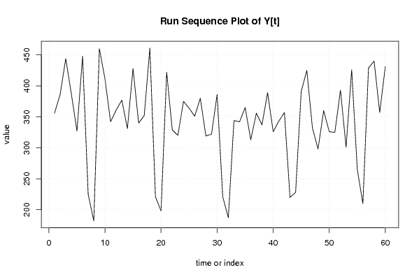
| Dataseries Y: | |||||||||||||||||||||||||||||||||||||||||||||||||||||||||||||||||
356 386 444 387 327 448 225 182 460 411 342 361 377 331 428 340 352 461 221 198 422 329 320 375 364 351 380 319 322 386 221 187 344 342 365 313 356 337 389 326 343 357 220 228 391 425 332 298 360 326 325 393 301 426 265 210 429 440 357 431 | |||||||||||||||||||||||||||||||||||||||||||||||||||||||||||||||||
Tables (Output of Computation) | |||||||||||||||||||||||||||||||||||||||||||||||||||||||||||||||||
| |||||||||||||||||||||||||||||||||||||||||||||||||||||||||||||||||
Figures (Output of Computation) | |||||||||||||||||||||||||||||||||||||||||||||||||||||||||||||||||
Input Parameters & R Code | |||||||||||||||||||||||||||||||||||||||||||||||||||||||||||||||||
| Parameters (Session): | |||||||||||||||||||||||||||||||||||||||||||||||||||||||||||||||||
| par1 = 0 ; par2 = 1 ; | |||||||||||||||||||||||||||||||||||||||||||||||||||||||||||||||||
| Parameters (R input): | |||||||||||||||||||||||||||||||||||||||||||||||||||||||||||||||||
| par1 = 0 ; par2 = 1 ; | |||||||||||||||||||||||||||||||||||||||||||||||||||||||||||||||||
| R code (references can be found in the software module): | |||||||||||||||||||||||||||||||||||||||||||||||||||||||||||||||||
par1 <- as.numeric(par1) | |||||||||||||||||||||||||||||||||||||||||||||||||||||||||||||||||