Free Statistics
of Irreproducible Research!
Description of Statistical Computation | |||||||||||||||||||||
|---|---|---|---|---|---|---|---|---|---|---|---|---|---|---|---|---|---|---|---|---|---|
| Author's title | |||||||||||||||||||||
| Author | *The author of this computation has been verified* | ||||||||||||||||||||
| R Software Module | rwasp_cloud.wasp | ||||||||||||||||||||
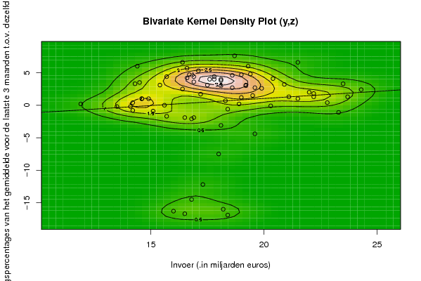
| Title produced by software | Trivariate Scatterplots | ||||||||||||||||||||
| Date of computation | Wed, 28 Oct 2009 11:50:21 -0600 | ||||||||||||||||||||
| Cite this page as follows | Statistical Computations at FreeStatistics.org, Office for Research Development and Education, URL https://freestatistics.org/blog/index.php?v=date/2009/Oct/28/t12567522887vsxw6vd5ngpsd8.htm/, Retrieved Sun, 05 May 2024 21:09:18 +0000 | ||||||||||||||||||||
| Statistical Computations at FreeStatistics.org, Office for Research Development and Education, URL https://freestatistics.org/blog/index.php?pk=51657, Retrieved Sun, 05 May 2024 21:09:18 +0000 | |||||||||||||||||||||
| QR Codes: | |||||||||||||||||||||
|
| |||||||||||||||||||||
| Original text written by user: | |||||||||||||||||||||
| IsPrivate? | No (this computation is public) | ||||||||||||||||||||
| User-defined keywords | SHW WS 5 -Trivariate scatterplots | ||||||||||||||||||||
| Estimated Impact | 137 | ||||||||||||||||||||
Tree of Dependent Computations | |||||||||||||||||||||
| Family? (F = Feedback message, R = changed R code, M = changed R Module, P = changed Parameters, D = changed Data) | |||||||||||||||||||||
| - [Trivariate Scatterplots] [WS 5 -Trivariate ...] [2009-10-28 17:50:21] [a45cc820faa25ce30779915639528ec2] [Current] - MPD [Trivariate Scatterplots] [Paper: Trivariate...] [2009-12-17 12:05:12] [b103a1dc147def8132c7f643ad8c8f84] | |||||||||||||||||||||
| Feedback Forum | |||||||||||||||||||||
Post a new message | |||||||||||||||||||||
Dataset | |||||||||||||||||||||
| Dataseries X: | |||||||||||||||||||||
15.5 15.1 11.7 16.3 16.7 15 14.9 14.6 15.3 17.9 16.4 15.4 17.9 15.9 13.9 17.8 17.9 17.4 16.7 16 16.6 19.1 17.8 17.2 18.6 16.3 15.1 19.2 17.7 19.1 18 17.5 17.8 21.1 17.2 19.4 19.8 17.6 16.2 19.5 19.9 20 17.3 18.9 18.6 21.4 18.6 19.8 20.8 19.6 17.7 19.8 22.2 20.7 17.9 20.9 21.2 21.4 23 21.3 23.9 22.4 18.3 22.8 22.3 17.8 16.4 16 16.4 17.7 16.6 16.2 18.3 | |||||||||||||||||||||
| Dataseries Y: | |||||||||||||||||||||
14.2 13.5 11.9 14.6 15.6 14.1 14.9 14.2 14.6 17.2 15.4 14.3 17.5 14.5 14.4 16.6 16.7 16.6 16.9 15.7 16.4 18.4 16.9 16.5 18.3 15.1 15.7 18.1 16.8 18.9 19 18.1 17.8 21.5 17.1 18.7 19 16.4 16.9 18.6 19.3 19.4 17.6 18.6 18.1 20.4 18.1 19.6 19.9 19.2 17.8 19.2 22 21.1 19.5 22.2 20.9 22.2 23.5 21.5 24.3 22.8 20.3 23.7 23.3 19.6 18 17.3 16.8 18.2 16.5 16 18.4 | |||||||||||||||||||||
| Dataseries Z: | |||||||||||||||||||||
-0.8 -0.2 0.2 1 0 -0.2 1 0.4 1 1.7 3.1 3.3 3.1 3.5 6 5.7 4.7 4.2 3.6 4.4 2.5 -0.6 -1.9 -1.9 0.7 -0.9 -1.7 -3.1 -2.1 0.2 1.2 3.8 4 6.6 5.3 7.6 4.7 6.6 4.4 4.6 6 4.8 4 2.7 3 4.1 4 2.7 2.6 3.1 4.4 3 2 1.3 1.5 1.3 3.2 1.8 3.3 1 2.4 0.4 -0.1 1.3 -1.1 -4.4 -7.5 -12.2 -14.5 -16 -16.7 -16.3 -16.9 | |||||||||||||||||||||
Tables (Output of Computation) | |||||||||||||||||||||
| |||||||||||||||||||||
Figures (Output of Computation) | |||||||||||||||||||||
Input Parameters & R Code | |||||||||||||||||||||
| Parameters (Session): | |||||||||||||||||||||
| par1 = 50 ; par2 = 50 ; par3 = Y ; par4 = Y ; par5 = Uitvoer (in miljarden euros) ; par6 = Invoer (�in miljarden euros) ; par7 = Industri�le productie (veranderingspercentages van het gemiddelde voor de laatste 3 maanden t.o.v. dezelfde periode van het voorgaande jaar) ; | |||||||||||||||||||||
| Parameters (R input): | |||||||||||||||||||||
| par1 = 50 ; par2 = 50 ; par3 = Y ; par4 = Y ; par5 = Uitvoer (in miljarden euros) ; par6 = Invoer (�in miljarden euros) ; par7 = Industri�le productie (veranderingspercentages van het gemiddelde voor de laatste 3 maanden t.o.v. dezelfde periode van het voorgaande jaar) ; | |||||||||||||||||||||
| R code (references can be found in the software module): | |||||||||||||||||||||
x <- array(x,dim=c(length(x),1)) | |||||||||||||||||||||