Free Statistics
of Irreproducible Research!
Description of Statistical Computation | |||||||||||||||||||||||||||||||||||||||||||||||||||||||||||||||||
|---|---|---|---|---|---|---|---|---|---|---|---|---|---|---|---|---|---|---|---|---|---|---|---|---|---|---|---|---|---|---|---|---|---|---|---|---|---|---|---|---|---|---|---|---|---|---|---|---|---|---|---|---|---|---|---|---|---|---|---|---|---|---|---|---|---|
| Author's title | |||||||||||||||||||||||||||||||||||||||||||||||||||||||||||||||||
| Author | *The author of this computation has been verified* | ||||||||||||||||||||||||||||||||||||||||||||||||||||||||||||||||
| R Software Module | rwasp_edabi.wasp | ||||||||||||||||||||||||||||||||||||||||||||||||||||||||||||||||
| Title produced by software | Bivariate Explorative Data Analysis | ||||||||||||||||||||||||||||||||||||||||||||||||||||||||||||||||
| Date of computation | Wed, 28 Oct 2009 10:44:36 -0600 | ||||||||||||||||||||||||||||||||||||||||||||||||||||||||||||||||
| Cite this page as follows | Statistical Computations at FreeStatistics.org, Office for Research Development and Education, URL https://freestatistics.org/blog/index.php?v=date/2009/Oct/28/t1256748520tcjg5rmycynfc25.htm/, Retrieved Mon, 06 May 2024 04:05:00 +0000 | ||||||||||||||||||||||||||||||||||||||||||||||||||||||||||||||||
| Statistical Computations at FreeStatistics.org, Office for Research Development and Education, URL https://freestatistics.org/blog/index.php?pk=51547, Retrieved Mon, 06 May 2024 04:05:00 +0000 | |||||||||||||||||||||||||||||||||||||||||||||||||||||||||||||||||
| QR Codes: | |||||||||||||||||||||||||||||||||||||||||||||||||||||||||||||||||
|
| |||||||||||||||||||||||||||||||||||||||||||||||||||||||||||||||||
| Original text written by user: | |||||||||||||||||||||||||||||||||||||||||||||||||||||||||||||||||
| IsPrivate? | No (this computation is public) | ||||||||||||||||||||||||||||||||||||||||||||||||||||||||||||||||
| User-defined keywords | shwws4v2 | ||||||||||||||||||||||||||||||||||||||||||||||||||||||||||||||||
| Estimated Impact | 137 | ||||||||||||||||||||||||||||||||||||||||||||||||||||||||||||||||
Tree of Dependent Computations | |||||||||||||||||||||||||||||||||||||||||||||||||||||||||||||||||
| Family? (F = Feedback message, R = changed R code, M = changed R Module, P = changed Parameters, D = changed Data) | |||||||||||||||||||||||||||||||||||||||||||||||||||||||||||||||||
| - [Bivariate Data Series] [Bivariate dataset] [2008-01-05 23:51:08] [74be16979710d4c4e7c6647856088456] - RMPD [Bivariate Explorative Data Analysis] [] [2009-10-28 15:16:32] [5482608004c1d7bbf873930172393a2d] - D [Bivariate Explorative Data Analysis] [] [2009-10-28 16:44:36] [efdfe680cd785c4af09f858b30f777ec] [Current] - RMPD [Trivariate Scatterplots] [] [2009-11-03 17:57:36] [5482608004c1d7bbf873930172393a2d] - RMPD [Bivariate Explorative Data Analysis] [] [2009-11-03 18:16:45] [5482608004c1d7bbf873930172393a2d] - [Bivariate Explorative Data Analysis] [Workshop 5, Bivar...] [2009-11-04 10:51:00] [aba88da643e3763d32ff92bd8f92a385] - D [Bivariate Explorative Data Analysis] [Workshop 5 Bivari...] [2009-11-04 10:53:38] [b6394cb5c2dcec6d17418d3cdf42d699] - D [Bivariate Explorative Data Analysis] [workshop 5 bivari...] [2009-11-04 10:53:21] [af8eb90b4bf1bcfcc4325c143dbee260] - D [Bivariate Explorative Data Analysis] [Workshop 5, Bivar...] [2009-11-04 10:55:14] [b03a417d80508f12cef0f78b0fc3a1dd] - D [Bivariate Explorative Data Analysis] [Workshop 5, Bivar...] [2009-11-04 10:55:14] [aba88da643e3763d32ff92bd8f92a385] - RMPD [Bivariate Explorative Data Analysis] [] [2009-11-03 18:19:20] [5482608004c1d7bbf873930172393a2d] - D [Bivariate Explorative Data Analysis] [Workshop 5 Bivari...] [2009-11-04 10:59:12] [b6394cb5c2dcec6d17418d3cdf42d699] - D [Bivariate Explorative Data Analysis] [workshop 5 bivari...] [2009-11-04 10:59:07] [af8eb90b4bf1bcfcc4325c143dbee260] - D [Bivariate Explorative Data Analysis] [Workshop 5, Bivar...] [2009-11-04 10:59:59] [aba88da643e3763d32ff92bd8f92a385] - RMPD [Bivariate Explorative Data Analysis] [] [2009-11-03 18:33:00] [5482608004c1d7bbf873930172393a2d] - D [Bivariate Explorative Data Analysis] [workshop 5 bivari...] [2009-11-04 11:34:19] [af8eb90b4bf1bcfcc4325c143dbee260] - D [Bivariate Explorative Data Analysis] [Workshop 5 Bivari...] [2009-11-04 11:34:29] [b6394cb5c2dcec6d17418d3cdf42d699] - D [Bivariate Explorative Data Analysis] [Workshop 5, Bivar...] [2009-11-04 11:44:07] [aba88da643e3763d32ff92bd8f92a385] - PD [Trivariate Scatterplots] [workshop 5 totale...] [2009-11-04 10:34:43] [af8eb90b4bf1bcfcc4325c143dbee260] - PD [Trivariate Scatterplots] [Workshop 5 Trivia...] [2009-11-04 10:33:16] [b6394cb5c2dcec6d17418d3cdf42d699] - PD [Trivariate Scatterplots] [Workshop 5, Triva...] [2009-11-04 10:37:52] [aba88da643e3763d32ff92bd8f92a385] - RMPD [Partial Correlation] [] [2009-11-03 18:08:02] [5482608004c1d7bbf873930172393a2d] - D [Partial Correlation] [Workshop 5, Parti...] [2009-11-04 10:44:56] [aba88da643e3763d32ff92bd8f92a385] - D [Partial Correlation] [Workshop 5 Partia...] [2009-11-04 10:47:33] [b6394cb5c2dcec6d17418d3cdf42d699] F D [Partial Correlation] [workshop 5 partia...] [2009-11-04 10:47:06] [af8eb90b4bf1bcfcc4325c143dbee260] - D [Partial Correlation] [WS5 Partial Corre...] [2009-11-04 16:44:56] [1b4c3bbe3f2ba180dd536c5a6a81a8e6] - RMPD [Bivariate Explorative Data Analysis] [WS5 Bivariate EDA...] [2009-11-04 17:16:47] [1b4c3bbe3f2ba180dd536c5a6a81a8e6] - RMPD [Bivariate Explorative Data Analysis] [WS5 Bivariate EDA...] [2009-11-04 17:21:54] [1b4c3bbe3f2ba180dd536c5a6a81a8e6] - RMPD [Bivariate Explorative Data Analysis] [WS5 Bivariate EDA...] [2009-11-04 17:21:54] [1b4c3bbe3f2ba180dd536c5a6a81a8e6] | |||||||||||||||||||||||||||||||||||||||||||||||||||||||||||||||||
| Feedback Forum | |||||||||||||||||||||||||||||||||||||||||||||||||||||||||||||||||
Post a new message | |||||||||||||||||||||||||||||||||||||||||||||||||||||||||||||||||
Dataset | |||||||||||||||||||||||||||||||||||||||||||||||||||||||||||||||||
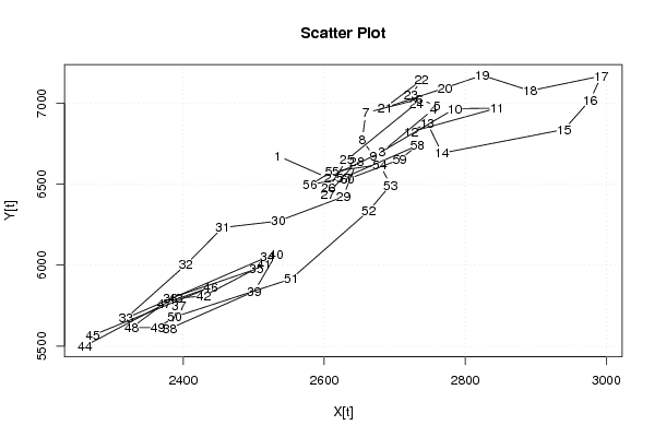
| Dataseries X: | |||||||||||||||||||||||||||||||||||||||||||||||||||||||||||||||||
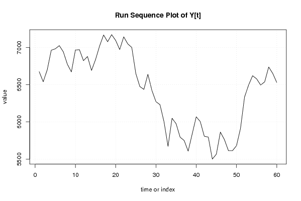
2534 2605 2682 2755 2760 2735 2659 2654 2670 2785 2845 2723 2746 2767 2940 2977 2993 2892 2824 2771 2686 2738 2723 2731 2632 2606 2605 2646 2627 2535 2456 2404 2319 2519 2504 2382 2394 2381 2501 2532 2515 2429 2389 2261 2272 2439 2373 2327 2364 2388 2553 2663 2694 2679 2611 2580 2627 2732 2707 2633 | |||||||||||||||||||||||||||||||||||||||||||||||||||||||||||||||||
| Dataseries Y: | |||||||||||||||||||||||||||||||||||||||||||||||||||||||||||||||||
6675 6539 6699 6962 6981 7024 6940 6774 6671 6965 6969 6822 6878 6691 6837 7018 7167 7076 7171 7093 6971 7142 7047 6999 6650 6475 6437 6639 6422 6272 6232 6003 5673 6050 5977 5796 5752 5609 5839 6069 6006 5809 5797 5502 5568 5864 5764 5615 5615 5681 5915 6334 6494 6620 6578 6495 6538 6737 6651 6530 | |||||||||||||||||||||||||||||||||||||||||||||||||||||||||||||||||
Tables (Output of Computation) | |||||||||||||||||||||||||||||||||||||||||||||||||||||||||||||||||
| |||||||||||||||||||||||||||||||||||||||||||||||||||||||||||||||||
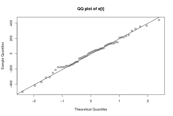
Figures (Output of Computation) | |||||||||||||||||||||||||||||||||||||||||||||||||||||||||||||||||
Input Parameters & R Code | |||||||||||||||||||||||||||||||||||||||||||||||||||||||||||||||||
| Parameters (Session): | |||||||||||||||||||||||||||||||||||||||||||||||||||||||||||||||||
| par1 = 0 ; par2 = 36 ; | |||||||||||||||||||||||||||||||||||||||||||||||||||||||||||||||||
| Parameters (R input): | |||||||||||||||||||||||||||||||||||||||||||||||||||||||||||||||||
| par1 = 0 ; par2 = 36 ; | |||||||||||||||||||||||||||||||||||||||||||||||||||||||||||||||||
| R code (references can be found in the software module): | |||||||||||||||||||||||||||||||||||||||||||||||||||||||||||||||||
par1 <- as.numeric(par1) | |||||||||||||||||||||||||||||||||||||||||||||||||||||||||||||||||