Free Statistics
of Irreproducible Research!
Description of Statistical Computation | |||||||||||||||||||||||||||||||||||||||||||||||||||||
|---|---|---|---|---|---|---|---|---|---|---|---|---|---|---|---|---|---|---|---|---|---|---|---|---|---|---|---|---|---|---|---|---|---|---|---|---|---|---|---|---|---|---|---|---|---|---|---|---|---|---|---|---|---|
| Author's title | |||||||||||||||||||||||||||||||||||||||||||||||||||||
| Author | *The author of this computation has been verified* | ||||||||||||||||||||||||||||||||||||||||||||||||||||
| R Software Module | rwasp_edauni.wasp | ||||||||||||||||||||||||||||||||||||||||||||||||||||
| Title produced by software | Univariate Explorative Data Analysis | ||||||||||||||||||||||||||||||||||||||||||||||||||||
| Date of computation | Tue, 27 Oct 2009 18:50:15 -0600 | ||||||||||||||||||||||||||||||||||||||||||||||||||||
| Cite this page as follows | Statistical Computations at FreeStatistics.org, Office for Research Development and Education, URL https://freestatistics.org/blog/index.php?v=date/2009/Oct/28/t1256691070sh9zk30ghdxagq0.htm/, Retrieved Sun, 05 May 2024 22:39:44 +0000 | ||||||||||||||||||||||||||||||||||||||||||||||||||||
| Statistical Computations at FreeStatistics.org, Office for Research Development and Education, URL https://freestatistics.org/blog/index.php?pk=51324, Retrieved Sun, 05 May 2024 22:39:44 +0000 | |||||||||||||||||||||||||||||||||||||||||||||||||||||
| QR Codes: | |||||||||||||||||||||||||||||||||||||||||||||||||||||
|
| |||||||||||||||||||||||||||||||||||||||||||||||||||||
| Original text written by user: | |||||||||||||||||||||||||||||||||||||||||||||||||||||
| IsPrivate? | No (this computation is public) | ||||||||||||||||||||||||||||||||||||||||||||||||||||
| User-defined keywords | |||||||||||||||||||||||||||||||||||||||||||||||||||||
| Estimated Impact | 170 | ||||||||||||||||||||||||||||||||||||||||||||||||||||
Tree of Dependent Computations | |||||||||||||||||||||||||||||||||||||||||||||||||||||
| Family? (F = Feedback message, R = changed R code, M = changed R Module, P = changed Parameters, D = changed Data) | |||||||||||||||||||||||||||||||||||||||||||||||||||||
| - [Bivariate Data Series] [Bivariate dataset] [2008-01-05 23:51:08] [74be16979710d4c4e7c6647856088456] - PD [Bivariate Data Series] [Reproduce: part 1] [2009-10-27 19:04:39] [f924a0adda9c1905a1ba8f1c751261ff] - RMP [Bivariate Explorative Data Analysis] [Bivariate EDA: Pa...] [2009-10-27 21:03:03] [f924a0adda9c1905a1ba8f1c751261ff] - D [Bivariate Explorative Data Analysis] [Bivariate EDA: Pa...] [2009-10-27 22:45:19] [f924a0adda9c1905a1ba8f1c751261ff] - D [Bivariate Explorative Data Analysis] [Bivariate data: P...] [2009-10-27 23:20:35] [f924a0adda9c1905a1ba8f1c751261ff] - RMPD [Harrell-Davis Quantiles] [Harell-Davis quan...] [2009-10-28 00:13:23] [f924a0adda9c1905a1ba8f1c751261ff] - RMPD [Univariate Explorative Data Analysis] [Unvariate EDA: pa...] [2009-10-28 00:50:15] [ac86848d66148c9c4c9404e0c9a511eb] [Current] | |||||||||||||||||||||||||||||||||||||||||||||||||||||
| Feedback Forum | |||||||||||||||||||||||||||||||||||||||||||||||||||||
Post a new message | |||||||||||||||||||||||||||||||||||||||||||||||||||||
Dataset | |||||||||||||||||||||||||||||||||||||||||||||||||||||
| Dataseries X: | |||||||||||||||||||||||||||||||||||||||||||||||||||||
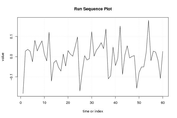
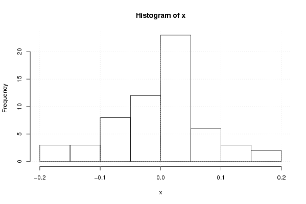
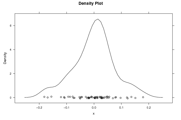
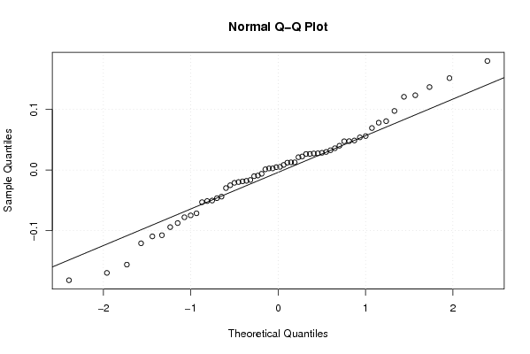
-0.181522675 0.027484233 0.035845163 0.02645656 -0.025079594 0.080434883 0.028309831 0.055884866 0.077929418 0.012619456 -0.021085382 0.120564813 -0.120699613 -0.029731785 -0.018707174 -0.052966034 -0.071292411 0.0125884 -0.046359987 0.029711131 0.01208106 0.002591969 0.048604574 0.097240699 -0.169416195 -0.074730702 0.004699456 -0.016414712 -0.010163004 0.123110568 0.002642395 0.032527273 0.047335339 0.069147875 0.039961483 0.136609601 -0.109306418 -0.094041885 0.04749451 -0.043852714 -0.00904968 0.151305062 -0.087388419 0.008380738 0.053715287 -0.006211395 0.001121426 0.005229885 -0.155813745 -0.077829277 -0.051105428 -0.050308314 0.021093937 0.17948073 -0.019811275 0.02719269 0.022338653 -0.017836631 -0.107377219 0.026367702 | |||||||||||||||||||||||||||||||||||||||||||||||||||||
Tables (Output of Computation) | |||||||||||||||||||||||||||||||||||||||||||||||||||||
| |||||||||||||||||||||||||||||||||||||||||||||||||||||
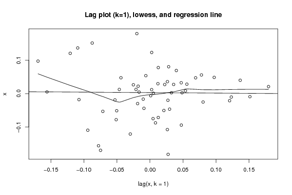
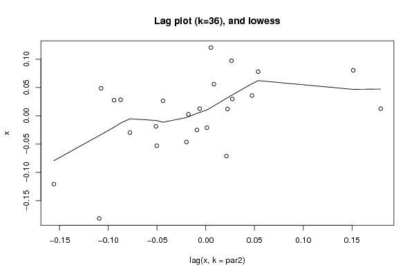
Figures (Output of Computation) | |||||||||||||||||||||||||||||||||||||||||||||||||||||
Input Parameters & R Code | |||||||||||||||||||||||||||||||||||||||||||||||||||||
| Parameters (Session): | |||||||||||||||||||||||||||||||||||||||||||||||||||||
| par1 = 0 ; par2 = 36 ; | |||||||||||||||||||||||||||||||||||||||||||||||||||||
| Parameters (R input): | |||||||||||||||||||||||||||||||||||||||||||||||||||||
| par1 = 0 ; par2 = 36 ; | |||||||||||||||||||||||||||||||||||||||||||||||||||||
| R code (references can be found in the software module): | |||||||||||||||||||||||||||||||||||||||||||||||||||||
par1 <- as.numeric(par1) | |||||||||||||||||||||||||||||||||||||||||||||||||||||