Free Statistics
of Irreproducible Research!
Description of Statistical Computation | |||||||||||||||||||||||||||||||||||||||||||||||||||||||||||||
|---|---|---|---|---|---|---|---|---|---|---|---|---|---|---|---|---|---|---|---|---|---|---|---|---|---|---|---|---|---|---|---|---|---|---|---|---|---|---|---|---|---|---|---|---|---|---|---|---|---|---|---|---|---|---|---|---|---|---|---|---|---|
| Author's title | |||||||||||||||||||||||||||||||||||||||||||||||||||||||||||||
| Author | *The author of this computation has been verified* | ||||||||||||||||||||||||||||||||||||||||||||||||||||||||||||
| R Software Module | rwasp_linear_regression.wasp | ||||||||||||||||||||||||||||||||||||||||||||||||||||||||||||
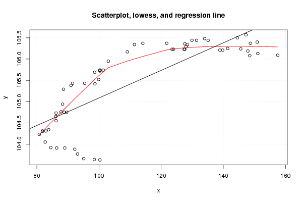
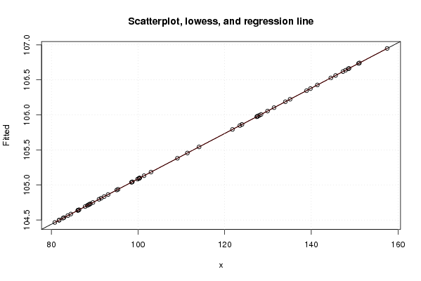
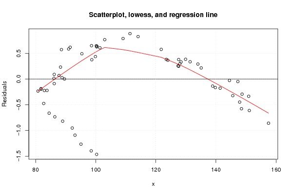
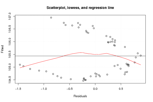
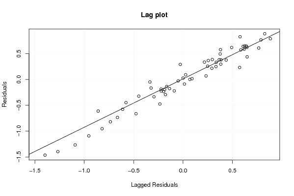
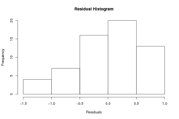
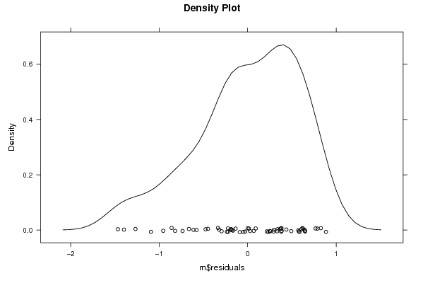
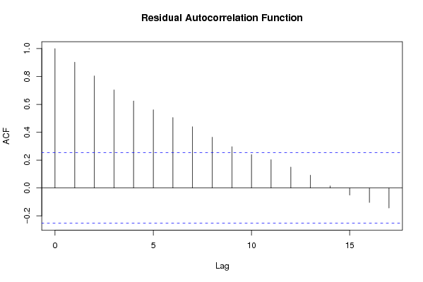
| Title produced by software | Linear Regression Graphical Model Validation | ||||||||||||||||||||||||||||||||||||||||||||||||||||||||||||
| Date of computation | Fri, 23 Oct 2009 10:51:23 -0600 | ||||||||||||||||||||||||||||||||||||||||||||||||||||||||||||
| Cite this page as follows | Statistical Computations at FreeStatistics.org, Office for Research Development and Education, URL https://freestatistics.org/blog/index.php?v=date/2009/Oct/23/t1256316724jqvk8igbf0b8kfz.htm/, Retrieved Thu, 02 May 2024 05:51:51 +0000 | ||||||||||||||||||||||||||||||||||||||||||||||||||||||||||||
| Statistical Computations at FreeStatistics.org, Office for Research Development and Education, URL https://freestatistics.org/blog/index.php?pk=50012, Retrieved Thu, 02 May 2024 05:51:51 +0000 | |||||||||||||||||||||||||||||||||||||||||||||||||||||||||||||
| QR Codes: | |||||||||||||||||||||||||||||||||||||||||||||||||||||||||||||
|
| |||||||||||||||||||||||||||||||||||||||||||||||||||||||||||||
| Original text written by user: | |||||||||||||||||||||||||||||||||||||||||||||||||||||||||||||
| IsPrivate? | No (this computation is public) | ||||||||||||||||||||||||||||||||||||||||||||||||||||||||||||
| User-defined keywords | |||||||||||||||||||||||||||||||||||||||||||||||||||||||||||||
| Estimated Impact | 157 | ||||||||||||||||||||||||||||||||||||||||||||||||||||||||||||
Tree of Dependent Computations | |||||||||||||||||||||||||||||||||||||||||||||||||||||||||||||
| Family? (F = Feedback message, R = changed R code, M = changed R Module, P = changed Parameters, D = changed Data) | |||||||||||||||||||||||||||||||||||||||||||||||||||||||||||||
| - [Bivariate Data Series] [Bivariate dataset] [2008-01-05 23:51:08] [74be16979710d4c4e7c6647856088456] - PD [Bivariate Data Series] [WS 4 1 PLOTS] [2009-10-23 11:13:05] [6e4e01d7eb22a9f33d58ebb35753a195] - RMPD [Bivariate Explorative Data Analysis] [ws 4 part 2] [2009-10-23 11:56:36] [6e4e01d7eb22a9f33d58ebb35753a195] - RMP [Pearson Correlation] [ws 4 2.1 r] [2009-10-23 12:05:33] [6e4e01d7eb22a9f33d58ebb35753a195] - RMP [Bivariate Kernel Density Estimation] [ws 4 p2.1] [2009-10-23 16:26:45] [6e4e01d7eb22a9f33d58ebb35753a195] - RMPD [Linear Regression Graphical Model Validation] [ws 2.2] [2009-10-23 16:47:44] [6e4e01d7eb22a9f33d58ebb35753a195] - D [Linear Regression Graphical Model Validation] [ws 2.2] [2009-10-23 16:51:23] [2e4ef2c1b76db9b31c0a03b96e94ad77] [Current] | |||||||||||||||||||||||||||||||||||||||||||||||||||||||||||||
| Feedback Forum | |||||||||||||||||||||||||||||||||||||||||||||||||||||||||||||
Post a new message | |||||||||||||||||||||||||||||||||||||||||||||||||||||||||||||
Dataset | |||||||||||||||||||||||||||||||||||||||||||||||||||||||||||||
| Dataseries X: | |||||||||||||||||||||||||||||||||||||||||||||||||||||||||||||
100,30 98,50 95,10 93,10 92,20 89,00 86,40 84,50 82,70 80,80 81,80 81,80 82,90 83,80 86,20 86,10 86,20 88,80 89,60 87,80 88,30 88,60 91,00 91,50 95,40 98,70 99,90 98,60 100,30 100,20 100,40 101,40 103,00 109,10 111,40 114,10 121,80 127,60 129,90 128,00 123,50 124,00 127,40 127,60 128,40 131,40 135,10 134,00 144,50 147,30 150,90 148,70 141,40 138,90 139,80 145,60 147,90 148,50 151,10 157,50 | |||||||||||||||||||||||||||||||||||||||||||||||||||||||||||||
| Dataseries Y: | |||||||||||||||||||||||||||||||||||||||||||||||||||||||||||||
103,63 103,64 103,66 103,77 103,88 103,91 103,91 103,92 104,05 104,23 104,30 104,31 104,31 104,34 104,55 104,65 104,73 104,75 104,75 104,76 104,94 105,29 105,38 105,43 105,43 105,42 105,52 105,69 105,72 105,74 105,74 105,74 105,95 106,17 106,34 106,37 106,37 106,36 106,44 106,29 106,23 106,23 106,23 106,23 106,34 106,44 106,44 106,48 106,50 106,57 106,40 106,37 106,25 106,21 106,21 106,24 106,19 106,08 106,13 106,09 | |||||||||||||||||||||||||||||||||||||||||||||||||||||||||||||
Tables (Output of Computation) | |||||||||||||||||||||||||||||||||||||||||||||||||||||||||||||
| |||||||||||||||||||||||||||||||||||||||||||||||||||||||||||||
Figures (Output of Computation) | |||||||||||||||||||||||||||||||||||||||||||||||||||||||||||||
Input Parameters & R Code | |||||||||||||||||||||||||||||||||||||||||||||||||||||||||||||
| Parameters (Session): | |||||||||||||||||||||||||||||||||||||||||||||||||||||||||||||
| par1 = 0 ; | |||||||||||||||||||||||||||||||||||||||||||||||||||||||||||||
| Parameters (R input): | |||||||||||||||||||||||||||||||||||||||||||||||||||||||||||||
| par1 = 0 ; | |||||||||||||||||||||||||||||||||||||||||||||||||||||||||||||
| R code (references can be found in the software module): | |||||||||||||||||||||||||||||||||||||||||||||||||||||||||||||
par1 <- as.numeric(par1) | |||||||||||||||||||||||||||||||||||||||||||||||||||||||||||||