Repository of Reproducible Computations

Free Statistics

of Irreproducible Research!

Author's title

Author

*The author of this computation has been verified*

R Software Module

rwasp_edauni.wasp

Title produced by software

Univariate Explorative Data Analysis

Date of computation

Fri, 23 Oct 2009 05:25:13 -0600

Cite this page as follows

Statistical Computations at FreeStatistics.org, Office for Research Development and Education, URL https://freestatistics.org/blog/index.php?v=date/2009/Oct/23/t1256297364ixniw04cvgo1pfh.htm/, Retrieved Thu, 02 May 2024 09:21:34 +0000

Statistical Computations at FreeStatistics.org, Office for Research Development and Education, URL https://freestatistics.org/blog/index.php?pk=49894, Retrieved Thu, 02 May 2024 09:21:34 +0000

QR Codes:

Paste this QR Code to cite your computation.

Original text written by user:

IsPrivate?

No (this computation is public)

User-defined keywords

Estimated Impact

162

Family? (F = Feedback message, R = changed R code, M = changed R Module, P = changed Parameters, D = changed Data)

-       [Univariate Explorative Data Analysis] [SHW_WS4_Q1_et] [2009-10-23 11:25:13] [f0f26816ac6124f58333f11f6c174000] [Current]
-    D    [Univariate Explorative Data Analysis] [] [2009-10-25 12:46:36] [08fc5c07292c885b941f0cb515ce13f3] 

Feedback Forum

Post a new message

Dataseries X:

Download CSV

Histogram

Boxplots

-71.29220372
-46.09220372
-26.04228392
13.57080222
47.3368745
60.87240621
56.62765671
49.84591314
44.72717551
39.65060224
29.02669431
24.81328737
20.59454974
17.45497053
15.62847746
4.32831706
-0.408677003
-8.382504729
-13.19316612
-27.48541068
-34.54098197
-36.89671366
-36.17603248
-36.27635328
-39.26875824
-40.38523152
-30.09182666
-32.30264845
-36.57841972
-39.04256721
-20.44968106
2.485369458
6.323807117
8.461282379
10.42234477
11.02266557
-1.153586908
6.26967942
0.42993981
-10.04518987
-5.945671065
-6.035651275
2.227194263
0.747875443
-8.594609714
-12.45034141
-24.16923944
-39.10753545
-41.59719486
-55.37392853
-59.36374834
-60.33773647
-61.50122361
-58.63320777
-60.28360877
-60.02350878
-59.11865929
-65.69863846
-73.37392853
-62.91899884
-62.58264637
-49.39621371
-54.48426912
-54.07376813
-51.64000082
-51.37731568
-52.61980084
-49.27553253
-48.96276719
-62.23919882
-60.08200478
-56.63531172
-52.63320777
-48.71268699
-45.82382958
-53.03627412
-52.79168501
-51.03174542
-49.82705633
-45.56453159
-52.5529078
-52.51058304
-49.42916028
-48.94030286
-43.93254742
-35.7989405
-36.26775833
-35.21250784
-33.28633557
-28.58924151
-23.26096529
-26.7050732
-26.3995821
-22.88439202
-22.58471282
-23.00280885
-20.3507851
-15.1462564
-17.37986332
-12.30489404
-7.96659803
-10.56062574
-6.540425756
-8.646398049
-13.1982614
-8.654313891
-15.79503465
-23.55820099
-13.55320985
52.62979816
45.99388939
36.59711614
30.85543298
29.57078346
25.21747652
14.57208541
-1.7128849
-1.239698772
0.426533911
3.123146765
2.951422988
-2.333386927
-5.115611693
-11.84517111
-18.97473053
-17.89895926
-18.48635432
-26.05000186
-20.23465137
-16.57875928
-31.61753649
-32.89427016
-23.01527214
-26.25130381
-29.62044244
-23.43062263
-24.01511174
-22.4579177
-13.53222662
-15.18020287
-11.5545118
-12.57761773
-16.8521058
-10.91849889
-7.147416708
7.232883264
7.571981275
3.274708069
11.18715261
10.07697242
16.85306449
14.21558923
9.770198126
4.451620895
-9.987637516
-3.585693967
-2.362748439
5.752281247
-5.294251408
-9.945954358
-1.533509819
5.331600067
15.77570797
15.83823271
4.054045642
6.064225833
0.160999087
2.505106993
5.262461437
9.98039707
-0.003290047
-3.743850409
-6.107497945
-5.27114548
-9.326877174
-15.27210788
-15.70958314
-17.56936233
-19.7459356
-22.20699799
-17.90699799
-8.982269315
-11.25673864
-11.94122775
-5.944133701
-8.228622816
1.469773188
3.73941177
-2.829245661
-6.297903092
-15.40339419
-17.07205162
-17.35121004
-6.467202122
-4.601611037
-7.908404082
-4.816159524
-1.626981313
0.793860267
-15.62716047
-15.31423473
-22.10130899
-19.78563771
-13.63070801
-7.765116927
-20.48064657
-58.06972064
-55.81495134
-52.36793749
-47.83595332
28.82140112
106.6244112
78.27251035
72.66571731
76.36297176
73.87703905
79.10515487
64.36266971
55.59337069
54.62988355
47.34958358
52.77447265
53.18417165
62.32473201
59.53200625
52.41747652
47.09647454
41.06222602
35.18324676
31.69487054
28.52362796
31.63817645
21.95691408
23.49326655
12.72072202
-15.35945506
-24.61390356
-28.17336195
-34.34702928
-17.65556796
-9.497071969
-42.87063516
-104.102109
-47.57736157
-71.21701579
-39.42751678
52.84013037
69.2609907
72.97473719
61.02758169
61.28074699
33.50754211
20.31271241
2.184096632
35.919845
25.4258173
38.48675679
32.17819935
28.85493303
24.42020331
31.52717551
22.84753589
10.74719634
5.158178525
6.305031979
10.96432997
13.60956068
15.33525175
21.2371953
13.72669431
24.62154277
30.11783482
34.35290409
43.30815459
12.52767546
-8.996109572
27.33945965
50.41362693
44.00619228
46.78601106
43.60394669
43.53061892
45.61995753
52.76827333
43.81528718
39.51576838
29.70316344
29.40252185
36.58799211
47.56426334
45.97750988
32.38412377
22.08314262
47.61548509
42.43374152
36.19189796
32.43438312
42.22664643
34.02001379
28.23277912
26.609994
30.31726824
12.09576631
18.14179901
32.58139697
30.05135636
46.67738698
45.266084
34.46574444
29.56574444
24.37768903
33.10888995
41.43698702
36.47850978
43.30872955
46.02035334
36.13941177
41.856385
35.82648603
38.92261769
37.8570266
30.68546323
24.5568662
31.4127583
21.36281974
17.24714846
20.42710888
21.76572569
11.1558663
-6.926056422
21.39933261
19.59448311
6.671037631
5.388973264
-15.93124547
-33.86665429
-7.984750323
-44.07897594
-62.870456
-26.04991647
-11.84586897
9.469660666
19.33657245
34.24707344
39.51348528
21.52024082
-0.804487859
-6.73340568
-35.22957484
-23.69933632
0.142846794
-2.911922502
9.178718059
2.95208334
0.268396223
-6.821121541
-2.288477022
-3.173286936
-23.60498781
-42.43328279

Summary of computational transaction
Raw Input	view raw input (R code)
Raw Output	view raw output of R engine
Computing time	4 seconds
R Server	'RServer@AstonUniversity' @ vre.aston.ac.uk

\begin{tabular}{lllllllll}
\hline
Summary of computational transaction \tabularnewline
Raw Input & view raw input (R code)  \tabularnewline
Raw Output & view raw output of R engine  \tabularnewline
Computing time & 4 seconds \tabularnewline
R Server & 'RServer@AstonUniversity' @ vre.aston.ac.uk \tabularnewline
\hline
\end{tabular}
%Source: https://freestatistics.org/blog/index.php?pk=49894&T=0

[TABLE]
[ROW][C]Summary of computational transaction[/C][/ROW]
[ROW][C]Raw Input[/C][C]view raw input (R code) [/C][/ROW]
[ROW][C]Raw Output[/C][C]view raw output of R engine [/C][/ROW]
[ROW][C]Computing time[/C][C]4 seconds[/C][/ROW]
[ROW][C]R Server[/C][C]'RServer@AstonUniversity' @ vre.aston.ac.uk[/C][/ROW]
[/TABLE]
Source: https://freestatistics.org/blog/index.php?pk=49894&T=0

Globally Unique Identifier (entire table): ba.freestatistics.org/blog/index.php?pk=49894&T=0

As an alternative you can also use a QR Code:

The GUIDs for individual cells are displayed in the table below:

Summary of computational transaction
Raw Input	view raw input (R code)
Raw Output	view raw output of R engine
Computing time	4 seconds
R Server	'RServer@AstonUniversity' @ vre.aston.ac.uk

Descriptive Statistics
# observations	360
minimum	-104.102109
Q1	-23.0059246725
median	-1.580245566
mean	-5.83333080913147e-11
Q3	28.30549133
maximum	106.6244112

\begin{tabular}{lllllllll}
\hline
Descriptive Statistics \tabularnewline
# observations & 360 \tabularnewline
minimum & -104.102109 \tabularnewline
Q1 & -23.0059246725 \tabularnewline
median & -1.580245566 \tabularnewline
mean & -5.83333080913147e-11 \tabularnewline
Q3 & 28.30549133 \tabularnewline
maximum & 106.6244112 \tabularnewline
\hline
\end{tabular}
%Source: https://freestatistics.org/blog/index.php?pk=49894&T=1

[TABLE]
[ROW][C]Descriptive Statistics[/C][/ROW]
[ROW][C]# observations[/C][C]360[/C][/ROW]
[ROW][C]minimum[/C][C]-104.102109[/C][/ROW]
[ROW][C]Q1[/C][C]-23.0059246725[/C][/ROW]
[ROW][C]median[/C][C]-1.580245566[/C][/ROW]
[ROW][C]mean[/C][C]-5.83333080913147e-11[/C][/ROW]
[ROW][C]Q3[/C][C]28.30549133[/C][/ROW]
[ROW][C]maximum[/C][C]106.6244112[/C][/ROW]
[/TABLE]
Source: https://freestatistics.org/blog/index.php?pk=49894&T=1

Globally Unique Identifier (entire table): ba.freestatistics.org/blog/index.php?pk=49894&T=1

As an alternative you can also use a QR Code:

The GUIDs for individual cells are displayed in the table below:

Descriptive Statistics
# observations	360
minimum	-104.102109
Q1	-23.0059246725
median	-1.580245566
mean	-5.83333080913147e-11
Q3	28.30549133
maximum	106.6244112

Figure 1

PNG link

Postscript link

PDF link

Figure 2

PNG link

Postscript link

PDF link

Figure 3

PNG link

Postscript link

PDF link

Figure 4

PNG link

Postscript link

PDF link

Figure 5

PNG link

Postscript link

PDF link

Figure 6

PNG link

Postscript link

PDF link

Figure 7

PNG link

Postscript link

PDF link

Parameters (Session):

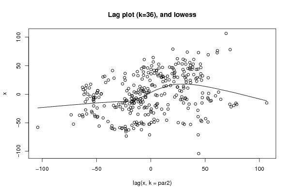
par1 = 0 ; par2 = 36 ;

Parameters (R input):

par1 = 0 ; par2 = 36 ;

R code (references can be found in the software module):

par1 <- as.numeric(par1)
par2 <- as.numeric(par2)
x <- as.ts(x)
library(lattice)
bitmap(file='pic1.png')
plot(x,type='l',main='Run Sequence Plot',xlab='time or index',ylab='value')
grid()
dev.off()
bitmap(file='pic2.png')
hist(x)
grid()
dev.off()
bitmap(file='pic3.png')
if (par1 > 0)
{
densityplot(~x,col='black',main=paste('Density Plot   bw = ',par1),bw=par1)
} else {
densityplot(~x,col='black',main='Density Plot')
}
dev.off()
bitmap(file='pic4.png')
qqnorm(x)
qqline(x)
grid()
dev.off()
if (par2 > 0)
{
bitmap(file='lagplot1.png')
dum <- cbind(lag(x,k=1),x)
dum
dum1 <- dum[2:length(x),]
dum1
z <- as.data.frame(dum1)
z
plot(z,main='Lag plot (k=1), lowess, and regression line')
lines(lowess(z))
abline(lm(z))
dev.off()
if (par2 > 1) {
bitmap(file='lagplotpar2.png')
dum <- cbind(lag(x,k=par2),x)
dum
dum1 <- dum[(par2+1):length(x),]
dum1
z <- as.data.frame(dum1)
z
mylagtitle <- 'Lag plot (k='
mylagtitle <- paste(mylagtitle,par2,sep='')
mylagtitle <- paste(mylagtitle,'), and lowess',sep='')
plot(z,main=mylagtitle)
lines(lowess(z))
dev.off()
}
bitmap(file='pic5.png')
acf(x,lag.max=par2,main='Autocorrelation Function')
grid()
dev.off()
}
summary(x)
load(file='createtable')
a<-table.start()
a<-table.row.start(a)
a<-table.element(a,'Descriptive Statistics',2,TRUE)
a<-table.row.end(a)
a<-table.row.start(a)
a<-table.element(a,'# observations',header=TRUE)
a<-table.element(a,length(x))
a<-table.row.end(a)
a<-table.row.start(a)
a<-table.element(a,'minimum',header=TRUE)
a<-table.element(a,min(x))
a<-table.row.end(a)
a<-table.row.start(a)
a<-table.element(a,'Q1',header=TRUE)
a<-table.element(a,quantile(x,0.25))
a<-table.row.end(a)
a<-table.row.start(a)
a<-table.element(a,'median',header=TRUE)
a<-table.element(a,median(x))
a<-table.row.end(a)
a<-table.row.start(a)
a<-table.element(a,'mean',header=TRUE)
a<-table.element(a,mean(x))
a<-table.row.end(a)
a<-table.row.start(a)
a<-table.element(a,'Q3',header=TRUE)
a<-table.element(a,quantile(x,0.75))
a<-table.row.end(a)
a<-table.row.start(a)
a<-table.element(a,'maximum',header=TRUE)
a<-table.element(a,max(x))
a<-table.row.end(a)
a<-table.end(a)
table.save(a,file='mytable.tab')

Free Statistics

Description of Statistical Computation

Tree of Dependent Computations

Dataset

Tables (Output of Computation)

Figures (Output of Computation)

Input Parameters & R Code