Free Statistics
of Irreproducible Research!
Description of Statistical Computation | |||||||||||||||||||||||||||||||||||||||||||||||||||||||||||||||||
|---|---|---|---|---|---|---|---|---|---|---|---|---|---|---|---|---|---|---|---|---|---|---|---|---|---|---|---|---|---|---|---|---|---|---|---|---|---|---|---|---|---|---|---|---|---|---|---|---|---|---|---|---|---|---|---|---|---|---|---|---|---|---|---|---|---|
| Author's title | |||||||||||||||||||||||||||||||||||||||||||||||||||||||||||||||||
| Author | *The author of this computation has been verified* | ||||||||||||||||||||||||||||||||||||||||||||||||||||||||||||||||
| R Software Module | rwasp_edabi.wasp | ||||||||||||||||||||||||||||||||||||||||||||||||||||||||||||||||
| Title produced by software | Bivariate Explorative Data Analysis | ||||||||||||||||||||||||||||||||||||||||||||||||||||||||||||||||
| Date of computation | Fri, 23 Oct 2009 03:15:48 -0600 | ||||||||||||||||||||||||||||||||||||||||||||||||||||||||||||||||
| Cite this page as follows | Statistical Computations at FreeStatistics.org, Office for Research Development and Education, URL https://freestatistics.org/blog/index.php?v=date/2009/Oct/23/t1256289478hz2h0z6grqnlphk.htm/, Retrieved Wed, 01 May 2024 23:15:42 +0000 | ||||||||||||||||||||||||||||||||||||||||||||||||||||||||||||||||
| Statistical Computations at FreeStatistics.org, Office for Research Development and Education, URL https://freestatistics.org/blog/index.php?pk=49857, Retrieved Wed, 01 May 2024 23:15:42 +0000 | |||||||||||||||||||||||||||||||||||||||||||||||||||||||||||||||||
| QR Codes: | |||||||||||||||||||||||||||||||||||||||||||||||||||||||||||||||||
|
| |||||||||||||||||||||||||||||||||||||||||||||||||||||||||||||||||
| Original text written by user: | |||||||||||||||||||||||||||||||||||||||||||||||||||||||||||||||||
| IsPrivate? | No (this computation is public) | ||||||||||||||||||||||||||||||||||||||||||||||||||||||||||||||||
| User-defined keywords | |||||||||||||||||||||||||||||||||||||||||||||||||||||||||||||||||
| Estimated Impact | 208 | ||||||||||||||||||||||||||||||||||||||||||||||||||||||||||||||||
Tree of Dependent Computations | |||||||||||||||||||||||||||||||||||||||||||||||||||||||||||||||||
| Family? (F = Feedback message, R = changed R code, M = changed R Module, P = changed Parameters, D = changed Data) | |||||||||||||||||||||||||||||||||||||||||||||||||||||||||||||||||
| - [Bivariate Data Series] [Bivariate dataset] [2008-01-05 23:51:08] [74be16979710d4c4e7c6647856088456] - RMPD [Bivariate Explorative Data Analysis] [WS4 Part2 Vraag1] [2009-10-23 09:15:48] [37de18e38c1490dd77c2b362ed87f3bb] [Current] - PD [Bivariate Explorative Data Analysis] [WS4 Part2 Vraag2] [2009-10-23 09:20:24] [42ad1186d39724f834063794eac7cea3] - PD [Bivariate Explorative Data Analysis] [WS4 Part2 Vraag3] [2009-10-23 09:26:27] [42ad1186d39724f834063794eac7cea3] - PD [Bivariate Explorative Data Analysis] [WS4 Part2 Vraag2 TVD] [2009-10-23 09:31:37] [42ad1186d39724f834063794eac7cea3] - P [Bivariate Explorative Data Analysis] [BDM 5] [2009-10-27 14:58:17] [f5d341d4bbba73282fc6e80153a6d315] - P [Bivariate Explorative Data Analysis] [TG 5] [2009-10-27 15:06:55] [a21bac9c8d3d56fdec8be4e719e2c7ed] - PD [Bivariate Explorative Data Analysis] [WS4 Part2 Vraag3 TVD] [2009-10-23 09:35:21] [42ad1186d39724f834063794eac7cea3] - P [Bivariate Explorative Data Analysis] [BDM 6] [2009-10-27 14:59:24] [f5d341d4bbba73282fc6e80153a6d315] - P [Bivariate Explorative Data Analysis] [TG 6] [2009-10-27 15:07:56] [a21bac9c8d3d56fdec8be4e719e2c7ed] - P [Bivariate Explorative Data Analysis] [BDM 4] [2009-10-27 14:57:01] [f5d341d4bbba73282fc6e80153a6d315] - MP [Bivariate Explorative Data Analysis] [tg12] [2009-11-10 14:39:34] [a21bac9c8d3d56fdec8be4e719e2c7ed] - R P [Bivariate Explorative Data Analysis] [ws6] [2009-11-15 22:36:29] [3fc64fd7a52ce121dfe13dba27bf6e5b] - MP [Bivariate Explorative Data Analysis] [TVD12] [2009-11-10 22:34:49] [42ad1186d39724f834063794eac7cea3] - P [Bivariate Explorative Data Analysis] [PA12] [2009-12-15 09:59:55] [a21bac9c8d3d56fdec8be4e719e2c7ed] - MPD [Bivariate Explorative Data Analysis] [WS6 EDA] [2009-11-12 16:38:11] [445b292c553470d9fed8bc2796fd3a00] - P [Bivariate Explorative Data Analysis] [TG 4] [2009-10-27 15:05:45] [a21bac9c8d3d56fdec8be4e719e2c7ed] - MP [Bivariate Explorative Data Analysis] [P1] [2009-12-15 09:43:25] [f5d341d4bbba73282fc6e80153a6d315] | |||||||||||||||||||||||||||||||||||||||||||||||||||||||||||||||||
| Feedback Forum | |||||||||||||||||||||||||||||||||||||||||||||||||||||||||||||||||
Post a new message | |||||||||||||||||||||||||||||||||||||||||||||||||||||||||||||||||
Dataset | |||||||||||||||||||||||||||||||||||||||||||||||||||||||||||||||||
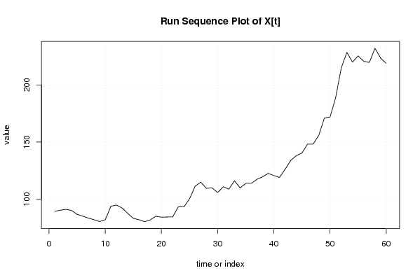
| Dataseries X: | |||||||||||||||||||||||||||||||||||||||||||||||||||||||||||||||||
89.3 90.3 91.1 90.1 86.7 85.1 83.4 82 80.4 81.9 93.8 94.8 92.3 87.5 83.2 82 80.3 81.8 85.1 84.2 84.4 84.5 93.3 93.2 100.3 111.4 114.9 109.5 109.9 105.8 110.8 108.8 116.1 109.8 113.8 113.8 117.4 119.5 122.6 120.7 119 126.1 133.9 138.1 140.4 148.2 148.2 155.9 171.1 171.9 188.8 214.9 228.5 220 225.4 220.7 219.7 232.1 223.5 218.9 | |||||||||||||||||||||||||||||||||||||||||||||||||||||||||||||||||
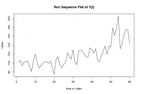
| Dataseries Y: | |||||||||||||||||||||||||||||||||||||||||||||||||||||||||||||||||
101.3 106.3 94 102.8 102 105.1 92.4 81.4 105.8 120.3 100.7 88.8 94.3 99.9 103.4 103.3 98.8 104.2 91.2 74.7 108.5 114.5 96.9 89.6 97.1 100.3 122.6 115.4 109 129.1 102.8 96.2 127.7 128.9 126.5 119.8 113.2 114.1 134.1 130 121.8 132.1 105.3 103 117.1 126.3 138.1 119.5 138 135.5 178.6 162.2 176.9 204.9 132.2 142.5 164.3 174.9 175.4 143 | |||||||||||||||||||||||||||||||||||||||||||||||||||||||||||||||||
Tables (Output of Computation) | |||||||||||||||||||||||||||||||||||||||||||||||||||||||||||||||||
| |||||||||||||||||||||||||||||||||||||||||||||||||||||||||||||||||
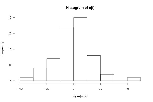
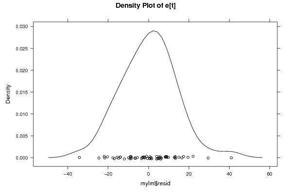
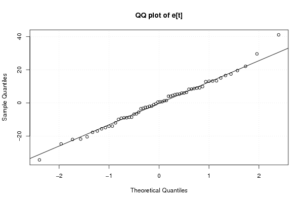
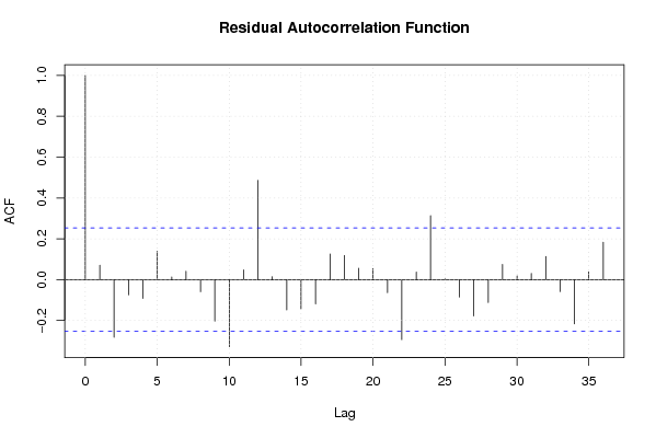
Figures (Output of Computation) | |||||||||||||||||||||||||||||||||||||||||||||||||||||||||||||||||
Input Parameters & R Code | |||||||||||||||||||||||||||||||||||||||||||||||||||||||||||||||||
| Parameters (Session): | |||||||||||||||||||||||||||||||||||||||||||||||||||||||||||||||||
| par1 = colombia ; par2 = www.ico.org ; par3 = Prices paid to growers in exporting Member countries in US cents per lb (Arabica, 1977/1 - 2006/12) ; par4 = usa ; par5 = www.ico.org ; par6 = Retail prices in importing Member countries in US cents per lb (Arabica, 1977/1 - 2006/12) ; | |||||||||||||||||||||||||||||||||||||||||||||||||||||||||||||||||
| Parameters (R input): | |||||||||||||||||||||||||||||||||||||||||||||||||||||||||||||||||
| par1 = 0 ; par2 = 36 ; | |||||||||||||||||||||||||||||||||||||||||||||||||||||||||||||||||
| R code (references can be found in the software module): | |||||||||||||||||||||||||||||||||||||||||||||||||||||||||||||||||
par1 <- as.numeric(par1) | |||||||||||||||||||||||||||||||||||||||||||||||||||||||||||||||||