Free Statistics
of Irreproducible Research!
Description of Statistical Computation | |||||||||||||||||||||||||||||||||||||||||||||||||||||
|---|---|---|---|---|---|---|---|---|---|---|---|---|---|---|---|---|---|---|---|---|---|---|---|---|---|---|---|---|---|---|---|---|---|---|---|---|---|---|---|---|---|---|---|---|---|---|---|---|---|---|---|---|---|
| Author's title | |||||||||||||||||||||||||||||||||||||||||||||||||||||
| Author | *The author of this computation has been verified* | ||||||||||||||||||||||||||||||||||||||||||||||||||||
| R Software Module | rwasp_edauni.wasp | ||||||||||||||||||||||||||||||||||||||||||||||||||||
| Title produced by software | Univariate Explorative Data Analysis | ||||||||||||||||||||||||||||||||||||||||||||||||||||
| Date of computation | Thu, 22 Oct 2009 14:33:00 -0600 | ||||||||||||||||||||||||||||||||||||||||||||||||||||
| Cite this page as follows | Statistical Computations at FreeStatistics.org, Office for Research Development and Education, URL https://freestatistics.org/blog/index.php?v=date/2009/Oct/22/t12562436517sisjn9zjtjpg5s.htm/, Retrieved Thu, 02 May 2024 21:10:10 +0000 | ||||||||||||||||||||||||||||||||||||||||||||||||||||
| Statistical Computations at FreeStatistics.org, Office for Research Development and Education, URL https://freestatistics.org/blog/index.php?pk=49822, Retrieved Thu, 02 May 2024 21:10:10 +0000 | |||||||||||||||||||||||||||||||||||||||||||||||||||||
| QR Codes: | |||||||||||||||||||||||||||||||||||||||||||||||||||||
|
| |||||||||||||||||||||||||||||||||||||||||||||||||||||
| Original text written by user: | |||||||||||||||||||||||||||||||||||||||||||||||||||||
| IsPrivate? | No (this computation is public) | ||||||||||||||||||||||||||||||||||||||||||||||||||||
| User-defined keywords | KVN WS3 | ||||||||||||||||||||||||||||||||||||||||||||||||||||
| Estimated Impact | 170 | ||||||||||||||||||||||||||||||||||||||||||||||||||||
Tree of Dependent Computations | |||||||||||||||||||||||||||||||||||||||||||||||||||||
| Family? (F = Feedback message, R = changed R code, M = changed R Module, P = changed Parameters, D = changed Data) | |||||||||||||||||||||||||||||||||||||||||||||||||||||
| - [Bivariate Data Series] [Bivariate dataset] [2008-01-05 23:51:08] [74be16979710d4c4e7c6647856088456] F RMPD [Univariate Explorative Data Analysis] [Colombia Coffee] [2008-01-07 14:21:11] [74be16979710d4c4e7c6647856088456] F RMPD [Univariate Data Series] [] [2009-10-14 08:30:28] [74be16979710d4c4e7c6647856088456] - RMPD [Central Tendency] [] [2009-10-20 15:12:09] [90f6d58d515a4caed6fb4b8be4e11eaa] - D [Central Tendency] [] [2009-10-20 15:25:16] [90f6d58d515a4caed6fb4b8be4e11eaa] - RMPD [Univariate Explorative Data Analysis] [] [2009-10-20 17:46:31] [90f6d58d515a4caed6fb4b8be4e11eaa] - D [Univariate Explorative Data Analysis] [WS3 Q2 Yt-Xt] [2009-10-22 20:33:00] [f1100e00818182135823a11ccbd0f3b9] [Current] - D [Univariate Explorative Data Analysis] [WS3 Q2 Yt-Xt Assu...] [2009-10-23 07:32:53] [1b4c3bbe3f2ba180dd536c5a6a81a8e6] | |||||||||||||||||||||||||||||||||||||||||||||||||||||
| Feedback Forum | |||||||||||||||||||||||||||||||||||||||||||||||||||||
Post a new message | |||||||||||||||||||||||||||||||||||||||||||||||||||||
Dataset | |||||||||||||||||||||||||||||||||||||||||||||||||||||
| Dataseries X: | |||||||||||||||||||||||||||||||||||||||||||||||||||||
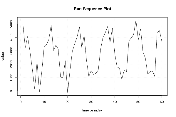
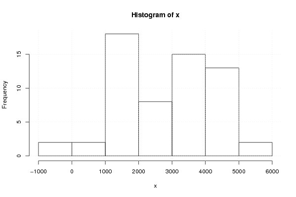
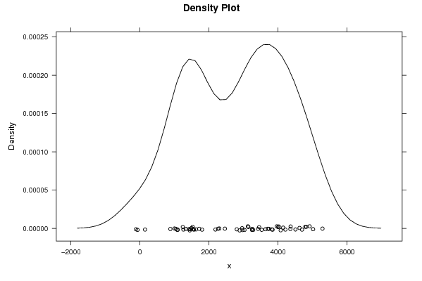
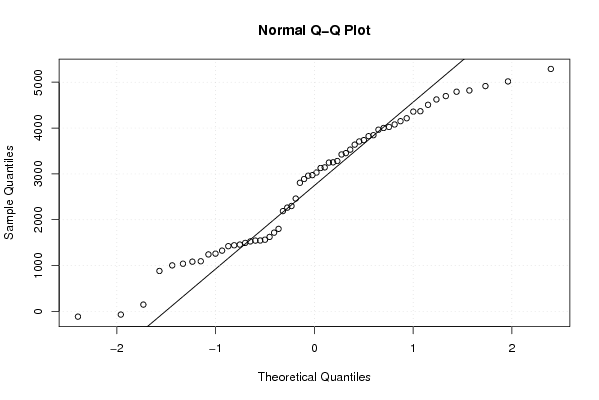
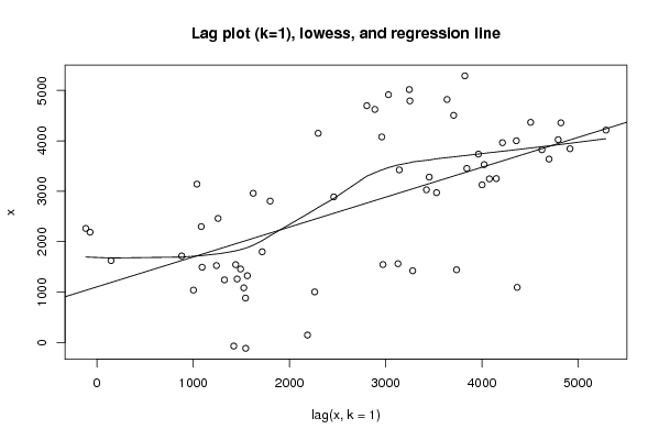
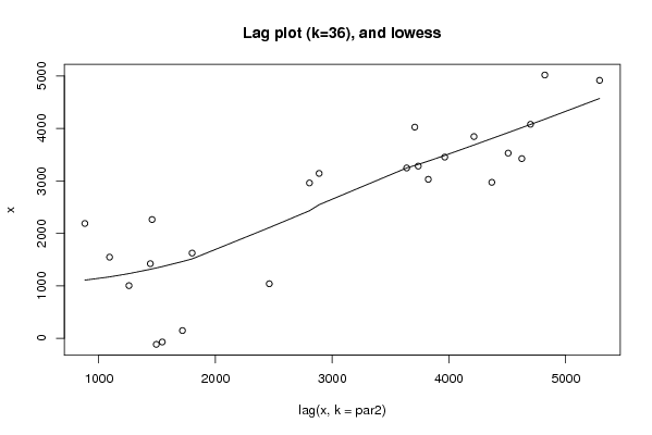
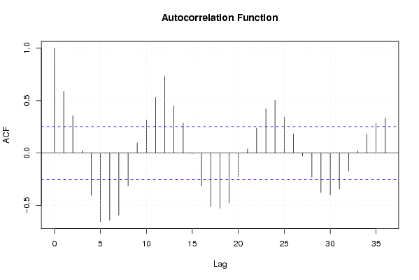
5018 3246 4078 2960 1624 147 2188 -71 1422 3281 3453 3844 4916 3029 3424 3142 1039 1003 2263 -116 1546 2972 3529 4024 4793 3252 4150 2299 1084 1526 1242 1325 1563 3128 4002 4358 4821 3638 4698 2805 1800 1717 881 1544 1442 3737 3964 4214 5290 3823 4624 2888 2461 1259 1457 1493 1093 4367 4507 3707 | |||||||||||||||||||||||||||||||||||||||||||||||||||||
Tables (Output of Computation) | |||||||||||||||||||||||||||||||||||||||||||||||||||||
| |||||||||||||||||||||||||||||||||||||||||||||||||||||
Figures (Output of Computation) | |||||||||||||||||||||||||||||||||||||||||||||||||||||
Input Parameters & R Code | |||||||||||||||||||||||||||||||||||||||||||||||||||||
| Parameters (Session): | |||||||||||||||||||||||||||||||||||||||||||||||||||||
| par1 = 0 ; par2 = 36 ; | |||||||||||||||||||||||||||||||||||||||||||||||||||||
| Parameters (R input): | |||||||||||||||||||||||||||||||||||||||||||||||||||||
| par1 = 0 ; par2 = 36 ; | |||||||||||||||||||||||||||||||||||||||||||||||||||||
| R code (references can be found in the software module): | |||||||||||||||||||||||||||||||||||||||||||||||||||||
par1 <- as.numeric(par1) | |||||||||||||||||||||||||||||||||||||||||||||||||||||