Free Statistics
of Irreproducible Research!
Description of Statistical Computation | |||||||||||||||||||||||||||||||||||||||||||||||||||||
|---|---|---|---|---|---|---|---|---|---|---|---|---|---|---|---|---|---|---|---|---|---|---|---|---|---|---|---|---|---|---|---|---|---|---|---|---|---|---|---|---|---|---|---|---|---|---|---|---|---|---|---|---|---|
| Author's title | |||||||||||||||||||||||||||||||||||||||||||||||||||||
| Author | *The author of this computation has been verified* | ||||||||||||||||||||||||||||||||||||||||||||||||||||
| R Software Module | rwasp_edauni.wasp | ||||||||||||||||||||||||||||||||||||||||||||||||||||
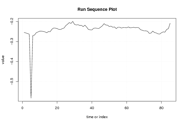
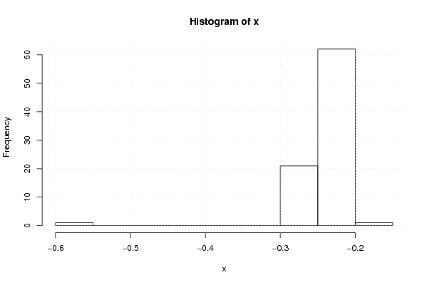
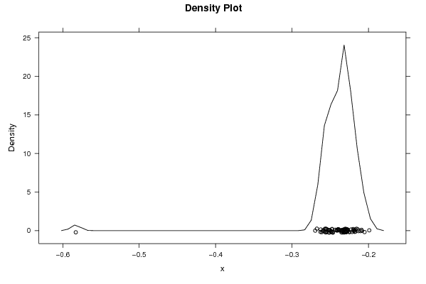
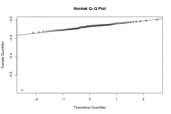
| Title produced by software | Univariate Explorative Data Analysis | ||||||||||||||||||||||||||||||||||||||||||||||||||||
| Date of computation | Tue, 20 Oct 2009 13:21:26 -0600 | ||||||||||||||||||||||||||||||||||||||||||||||||||||
| Cite this page as follows | Statistical Computations at FreeStatistics.org, Office for Research Development and Education, URL https://freestatistics.org/blog/index.php?v=date/2009/Oct/20/t1256066548dnrk0gtua65fe9m.htm/, Retrieved Thu, 02 May 2024 18:50:47 +0000 | ||||||||||||||||||||||||||||||||||||||||||||||||||||
| Statistical Computations at FreeStatistics.org, Office for Research Development and Education, URL https://freestatistics.org/blog/index.php?pk=49050, Retrieved Thu, 02 May 2024 18:50:47 +0000 | |||||||||||||||||||||||||||||||||||||||||||||||||||||
| QR Codes: | |||||||||||||||||||||||||||||||||||||||||||||||||||||
|
| |||||||||||||||||||||||||||||||||||||||||||||||||||||
| Original text written by user: | |||||||||||||||||||||||||||||||||||||||||||||||||||||
| IsPrivate? | No (this computation is public) | ||||||||||||||||||||||||||||||||||||||||||||||||||||
| User-defined keywords | workshop 3 deel 2.3 eda | ||||||||||||||||||||||||||||||||||||||||||||||||||||
| Estimated Impact | 122 | ||||||||||||||||||||||||||||||||||||||||||||||||||||
Tree of Dependent Computations | |||||||||||||||||||||||||||||||||||||||||||||||||||||
| Family? (F = Feedback message, R = changed R code, M = changed R Module, P = changed Parameters, D = changed Data) | |||||||||||||||||||||||||||||||||||||||||||||||||||||
| - [Bivariate Data Series] [Bivariate dataset] [2008-01-05 23:51:08] [74be16979710d4c4e7c6647856088456] F RMPD [Univariate Explorative Data Analysis] [Colombia Coffee] [2008-01-07 14:21:11] [74be16979710d4c4e7c6647856088456] F RMPD [Univariate Data Series] [] [2009-10-14 08:30:28] [74be16979710d4c4e7c6647856088456] - RMP [Histogram] [workshop 3 deel 1...] [2009-10-19 19:20:29] [309ee52d0058ff0a6f7eec15e07b2d9f] - RMPD [Univariate Explorative Data Analysis] [workshop 3 deel 2...] [2009-10-20 19:21:26] [6198946fb53eb5eb18db46bb758f7fde] [Current] | |||||||||||||||||||||||||||||||||||||||||||||||||||||
| Feedback Forum | |||||||||||||||||||||||||||||||||||||||||||||||||||||
Post a new message | |||||||||||||||||||||||||||||||||||||||||||||||||||||
Dataset | |||||||||||||||||||||||||||||||||||||||||||||||||||||
| Dataseries X: | |||||||||||||||||||||||||||||||||||||||||||||||||||||
-0,254448836 -0,256780831 -0,259858758 -0,262922664 -0,58299007 -0,269660681 -0,267500517 -0,255754535 -0,25189903 -0,247821188 -0,247866841 -0,249146156 -0,251426129 -0,25565253 -0,250103244 -0,250663359 -0,238473671 -0,232090754 -0,232847188 -0,234824571 -0,239128757 -0,239601826 -0,235402947 -0,232119695 -0,220166096 -0,213161853 -0,205117286 -0,209143249 -0,198978042 -0,213920482 -0,216990968 -0,215575519 -0,219207253 -0,219075142 -0,225220401 -0,217999529 -0,227524361 -0,239380179 -0,241235077 -0,241653918 -0,233510584 -0,232338549 -0,233602859 -0,234539434 -0,228081164 -0,221364739 -0,210459879 -0,217238843 -0,217936845 -0,224668866 -0,222757515 -0,228283207 -0,226825709 -0,234957874 -0,228228971 -0,228282532 -0,232320865 -0,22971766 -0,229870746 -0,230794044 -0,226855875 -0,231231714 -0,230266723 -0,228504068 -0,230569043 -0,229456547 -0,231130029 -0,24063145 -0,243416097 -0,246560656 -0,246300188 -0,248241127 -0,258941951 -0,257554536 -0,247733179 -0,254730878 -0,256799653 -0,261192655 -0,262520696 -0,255958914 -0,251464499 -0,252894413 -0,239531306 -0,235265203 -0,208414972 | |||||||||||||||||||||||||||||||||||||||||||||||||||||
Tables (Output of Computation) | |||||||||||||||||||||||||||||||||||||||||||||||||||||
| |||||||||||||||||||||||||||||||||||||||||||||||||||||
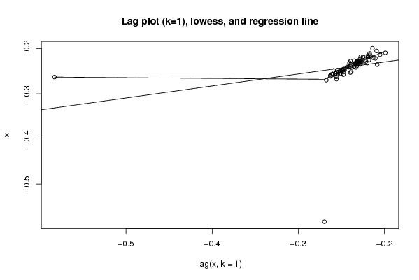
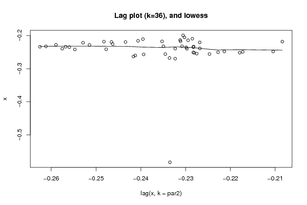
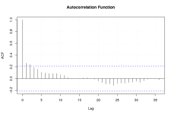
Figures (Output of Computation) | |||||||||||||||||||||||||||||||||||||||||||||||||||||
Input Parameters & R Code | |||||||||||||||||||||||||||||||||||||||||||||||||||||
| Parameters (Session): | |||||||||||||||||||||||||||||||||||||||||||||||||||||
| par1 = 0 ; par2 = 36 ; | |||||||||||||||||||||||||||||||||||||||||||||||||||||
| Parameters (R input): | |||||||||||||||||||||||||||||||||||||||||||||||||||||
| par1 = 0 ; par2 = 36 ; | |||||||||||||||||||||||||||||||||||||||||||||||||||||
| R code (references can be found in the software module): | |||||||||||||||||||||||||||||||||||||||||||||||||||||
par1 <- as.numeric(par1) | |||||||||||||||||||||||||||||||||||||||||||||||||||||