Free Statistics
of Irreproducible Research!
Description of Statistical Computation | |||||||||||||||||||||||||||||||||||||||||||||||||||||
|---|---|---|---|---|---|---|---|---|---|---|---|---|---|---|---|---|---|---|---|---|---|---|---|---|---|---|---|---|---|---|---|---|---|---|---|---|---|---|---|---|---|---|---|---|---|---|---|---|---|---|---|---|---|
| Author's title | |||||||||||||||||||||||||||||||||||||||||||||||||||||
| Author | *The author of this computation has been verified* | ||||||||||||||||||||||||||||||||||||||||||||||||||||
| R Software Module | rwasp_edauni.wasp | ||||||||||||||||||||||||||||||||||||||||||||||||||||
| Title produced by software | Univariate Explorative Data Analysis | ||||||||||||||||||||||||||||||||||||||||||||||||||||
| Date of computation | Tue, 20 Oct 2009 13:17:50 -0600 | ||||||||||||||||||||||||||||||||||||||||||||||||||||
| Cite this page as follows | Statistical Computations at FreeStatistics.org, Office for Research Development and Education, URL https://freestatistics.org/blog/index.php?v=date/2009/Oct/20/t1256066335o9pyfh5il15xc3r.htm/, Retrieved Thu, 02 May 2024 20:17:42 +0000 | ||||||||||||||||||||||||||||||||||||||||||||||||||||
| Statistical Computations at FreeStatistics.org, Office for Research Development and Education, URL https://freestatistics.org/blog/index.php?pk=49041, Retrieved Thu, 02 May 2024 20:17:42 +0000 | |||||||||||||||||||||||||||||||||||||||||||||||||||||
| QR Codes: | |||||||||||||||||||||||||||||||||||||||||||||||||||||
|
| |||||||||||||||||||||||||||||||||||||||||||||||||||||
| Original text written by user: | |||||||||||||||||||||||||||||||||||||||||||||||||||||
| IsPrivate? | No (this computation is public) | ||||||||||||||||||||||||||||||||||||||||||||||||||||
| User-defined keywords | workshop 3 deel 2.2 eda | ||||||||||||||||||||||||||||||||||||||||||||||||||||
| Estimated Impact | 145 | ||||||||||||||||||||||||||||||||||||||||||||||||||||
Tree of Dependent Computations | |||||||||||||||||||||||||||||||||||||||||||||||||||||
| Family? (F = Feedback message, R = changed R code, M = changed R Module, P = changed Parameters, D = changed Data) | |||||||||||||||||||||||||||||||||||||||||||||||||||||
| - [Bivariate Data Series] [Bivariate dataset] [2008-01-05 23:51:08] [74be16979710d4c4e7c6647856088456] F RMPD [Univariate Explorative Data Analysis] [Colombia Coffee] [2008-01-07 14:21:11] [74be16979710d4c4e7c6647856088456] F RMPD [Univariate Data Series] [] [2009-10-14 08:30:28] [74be16979710d4c4e7c6647856088456] - RMP [Histogram] [workshop 3 deel 1...] [2009-10-19 19:20:29] [309ee52d0058ff0a6f7eec15e07b2d9f] - RMPD [Univariate Explorative Data Analysis] [workshop 3 deel 2...] [2009-10-20 19:17:50] [6198946fb53eb5eb18db46bb758f7fde] [Current] | |||||||||||||||||||||||||||||||||||||||||||||||||||||
| Feedback Forum | |||||||||||||||||||||||||||||||||||||||||||||||||||||
Post a new message | |||||||||||||||||||||||||||||||||||||||||||||||||||||
Dataset | |||||||||||||||||||||||||||||||||||||||||||||||||||||
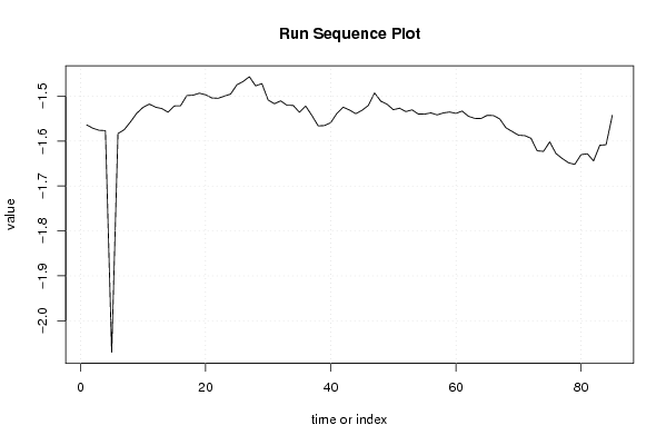
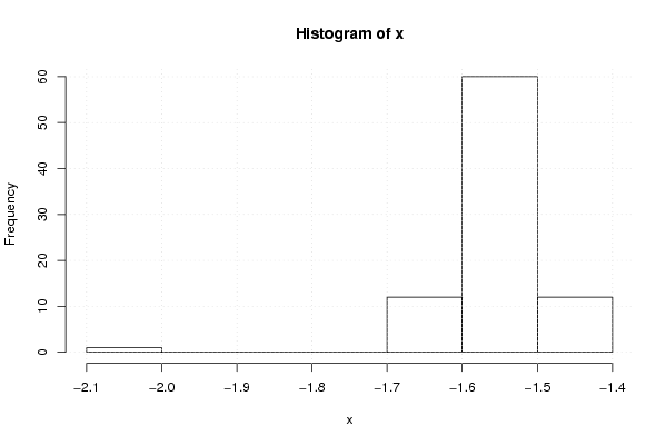
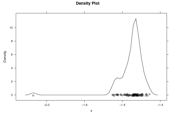
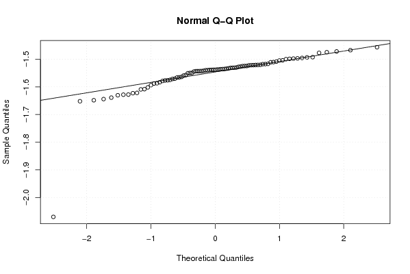
| Dataseries X: | |||||||||||||||||||||||||||||||||||||||||||||||||||||
-1,563895 -1,571395 -1,575945 -1,576615 -2,070195 -1,583195 -1,574525 -1,557275 -1,537985 -1,524965 -1,517515 -1,524375 -1,527505 -1,535495 -1,521665 -1,521325 -1,498565 -1,497645 -1,493295 -1,496865 -1,503905 -1,504655 -1,499805 -1,495325 -1,474585 -1,467225 -1,456545 -1,476975 -1,471875 -1,508455 -1,516745 -1,510405 -1,520065 -1,520465 -1,535815 -1,522035 -1,543145 -1,566095 -1,565355 -1,558975 -1,538025 -1,524515 -1,530835 -1,538875 -1,531395 -1,520755 -1,492575 -1,510995 -1,517825 -1,530015 -1,526665 -1,534165 -1,530405 -1,539745 -1,539835 -1,537125 -1,541595 -1,537225 -1,535165 -1,538275 -1,533015 -1,544625 -1,549345 -1,549765 -1,542695 -1,543035 -1,550475 -1,570405 -1,578585 -1,586855 -1,587825 -1,593635 -1,621685 -1,622795 -1,601785 -1,627755 -1,638835 -1,648275 -1,651895 -1,630235 -1,628225 -1,644055 -1,609135 -1,608155 -1,542645 | |||||||||||||||||||||||||||||||||||||||||||||||||||||
Tables (Output of Computation) | |||||||||||||||||||||||||||||||||||||||||||||||||||||
| |||||||||||||||||||||||||||||||||||||||||||||||||||||
Figures (Output of Computation) | |||||||||||||||||||||||||||||||||||||||||||||||||||||
Input Parameters & R Code | |||||||||||||||||||||||||||||||||||||||||||||||||||||
| Parameters (Session): | |||||||||||||||||||||||||||||||||||||||||||||||||||||
| par1 = 0 ; par2 = 36 ; | |||||||||||||||||||||||||||||||||||||||||||||||||||||
| Parameters (R input): | |||||||||||||||||||||||||||||||||||||||||||||||||||||
| par1 = 0 ; par2 = 36 ; | |||||||||||||||||||||||||||||||||||||||||||||||||||||
| R code (references can be found in the software module): | |||||||||||||||||||||||||||||||||||||||||||||||||||||
par1 <- as.numeric(par1) | |||||||||||||||||||||||||||||||||||||||||||||||||||||