Free Statistics
of Irreproducible Research!
Description of Statistical Computation | |||||||||||||||||||||||||||||||||||||||||||||||||||||
|---|---|---|---|---|---|---|---|---|---|---|---|---|---|---|---|---|---|---|---|---|---|---|---|---|---|---|---|---|---|---|---|---|---|---|---|---|---|---|---|---|---|---|---|---|---|---|---|---|---|---|---|---|---|
| Author's title | |||||||||||||||||||||||||||||||||||||||||||||||||||||
| Author | *The author of this computation has been verified* | ||||||||||||||||||||||||||||||||||||||||||||||||||||
| R Software Module | rwasp_edauni.wasp | ||||||||||||||||||||||||||||||||||||||||||||||||||||
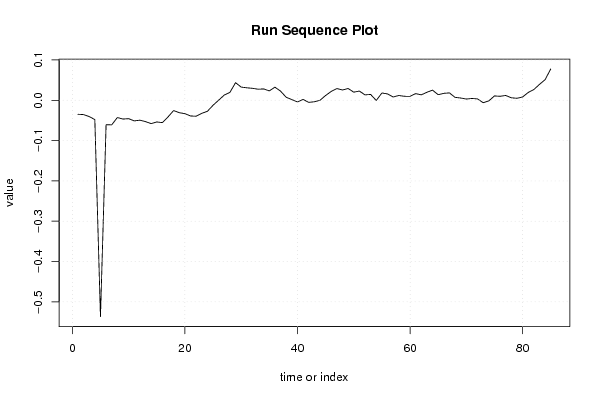
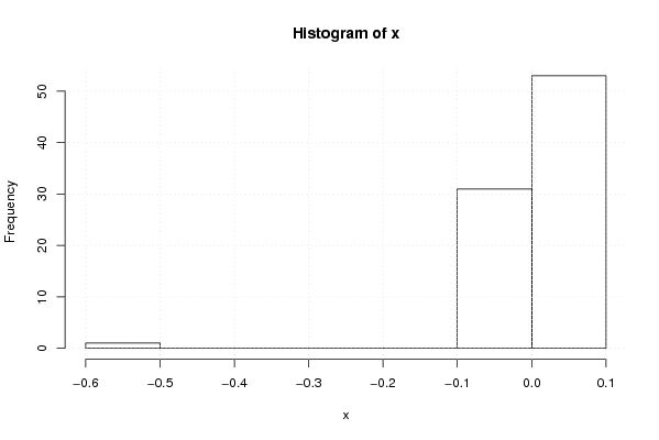
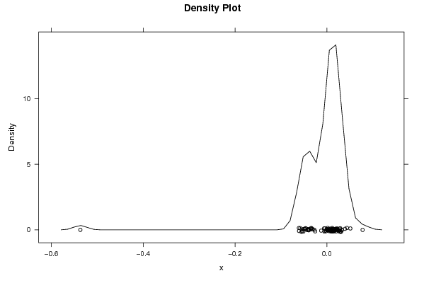
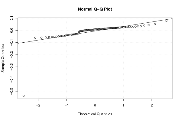
| Title produced by software | Univariate Explorative Data Analysis | ||||||||||||||||||||||||||||||||||||||||||||||||||||
| Date of computation | Tue, 20 Oct 2009 13:14:26 -0600 | ||||||||||||||||||||||||||||||||||||||||||||||||||||
| Cite this page as follows | Statistical Computations at FreeStatistics.org, Office for Research Development and Education, URL https://freestatistics.org/blog/index.php?v=date/2009/Oct/20/t12560661577z5agzgw0hrqzim.htm/, Retrieved Fri, 03 May 2024 03:42:30 +0000 | ||||||||||||||||||||||||||||||||||||||||||||||||||||
| Statistical Computations at FreeStatistics.org, Office for Research Development and Education, URL https://freestatistics.org/blog/index.php?pk=49032, Retrieved Fri, 03 May 2024 03:42:30 +0000 | |||||||||||||||||||||||||||||||||||||||||||||||||||||
| QR Codes: | |||||||||||||||||||||||||||||||||||||||||||||||||||||
|
| |||||||||||||||||||||||||||||||||||||||||||||||||||||
| Original text written by user: | |||||||||||||||||||||||||||||||||||||||||||||||||||||
| IsPrivate? | No (this computation is public) | ||||||||||||||||||||||||||||||||||||||||||||||||||||
| User-defined keywords | workshop 3 deel 2.1 eda | ||||||||||||||||||||||||||||||||||||||||||||||||||||
| Estimated Impact | 117 | ||||||||||||||||||||||||||||||||||||||||||||||||||||
Tree of Dependent Computations | |||||||||||||||||||||||||||||||||||||||||||||||||||||
| Family? (F = Feedback message, R = changed R code, M = changed R Module, P = changed Parameters, D = changed Data) | |||||||||||||||||||||||||||||||||||||||||||||||||||||
| - [Bivariate Data Series] [Bivariate dataset] [2008-01-05 23:51:08] [74be16979710d4c4e7c6647856088456] F RMPD [Univariate Explorative Data Analysis] [Colombia Coffee] [2008-01-07 14:21:11] [74be16979710d4c4e7c6647856088456] F RMPD [Univariate Data Series] [] [2009-10-14 08:30:28] [74be16979710d4c4e7c6647856088456] - RMP [Histogram] [workshop 3 deel 1...] [2009-10-19 19:20:29] [309ee52d0058ff0a6f7eec15e07b2d9f] - RMPD [Univariate Explorative Data Analysis] [workshop 3 deel 2...] [2009-10-20 19:14:26] [6198946fb53eb5eb18db46bb758f7fde] [Current] | |||||||||||||||||||||||||||||||||||||||||||||||||||||
| Feedback Forum | |||||||||||||||||||||||||||||||||||||||||||||||||||||
Post a new message | |||||||||||||||||||||||||||||||||||||||||||||||||||||
Dataset | |||||||||||||||||||||||||||||||||||||||||||||||||||||
| Dataseries X: | |||||||||||||||||||||||||||||||||||||||||||||||||||||
-0.034795 -0.035595 -0.040445 -0.047915 -0.536795 -0.060695 -0.061025 -0.042875 -0.046685 -0.045665 -0.051215 -0.049475 -0.053005 -0.057995 -0.053865 -0.055525 -0.041365 -0.025545 -0.030895 -0.033265 -0.039005 -0.039655 -0.032505 -0.027425 -0.012485 0.000175 0.012955 0.019425 0.043625 0.032645 0.030855 0.029595 0.027335 0.028035 0.023185 0.032365 0.022555 0.007305 0.001645 -0.004275 0.001975 -0.005315 -0.003835 -0.000175 0.011705 0.021845 0.029025 0.025405 0.029075 0.020085 0.022735 0.013335 0.014395 -0.000645 0.017965 0.015675 0.008005 0.011775 0.009735 0.009625 0.016385 0.013375 0.019755 0.025035 0.013705 0.017065 0.018225 0.007095 0.005515 0.002945 0.004375 0.003265 -0.006185 -0.001595 0.010615 0.009745 0.011765 0.006025 0.004805 0.008065 0.019275 0.026545 0.039365 0.051045 0.077655 | |||||||||||||||||||||||||||||||||||||||||||||||||||||
Tables (Output of Computation) | |||||||||||||||||||||||||||||||||||||||||||||||||||||
| |||||||||||||||||||||||||||||||||||||||||||||||||||||
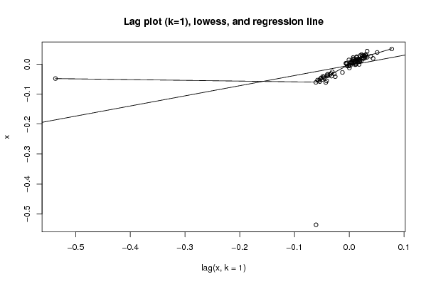
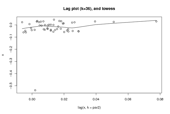
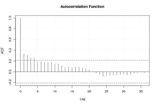
Figures (Output of Computation) | |||||||||||||||||||||||||||||||||||||||||||||||||||||
Input Parameters & R Code | |||||||||||||||||||||||||||||||||||||||||||||||||||||
| Parameters (Session): | |||||||||||||||||||||||||||||||||||||||||||||||||||||
| par1 = 0 ; par2 = 36 ; | |||||||||||||||||||||||||||||||||||||||||||||||||||||
| Parameters (R input): | |||||||||||||||||||||||||||||||||||||||||||||||||||||
| par1 = 0 ; par2 = 36 ; | |||||||||||||||||||||||||||||||||||||||||||||||||||||
| R code (references can be found in the software module): | |||||||||||||||||||||||||||||||||||||||||||||||||||||
par1 <- as.numeric(par1) | |||||||||||||||||||||||||||||||||||||||||||||||||||||