Repository of Reproducible Computations

Free Statistics

of Irreproducible Research!

Author's title

Author

*The author of this computation has been verified*

R Software Module

rwasp_edauni.wasp

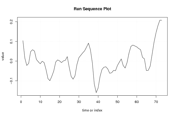
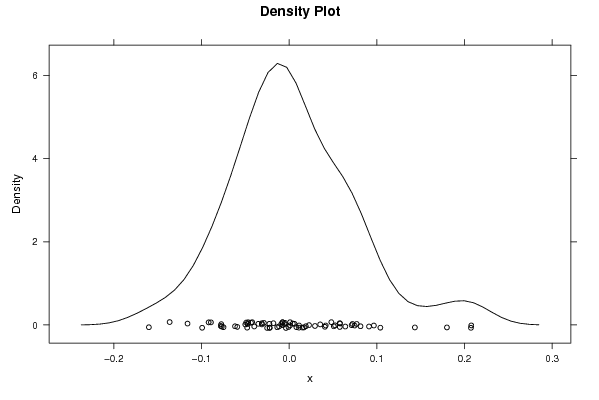
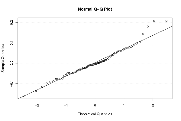
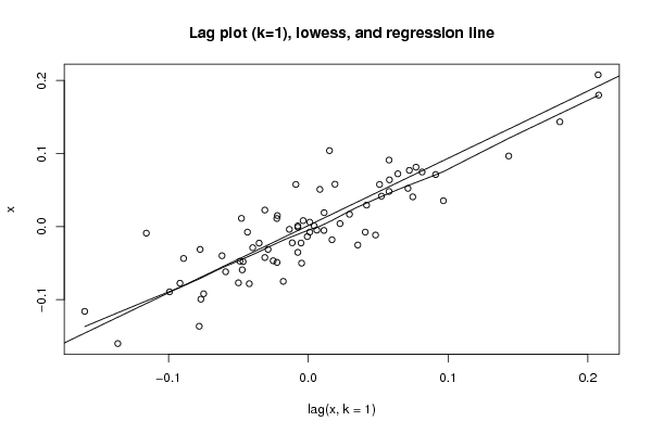
Title produced by software

Univariate Explorative Data Analysis

Date of computation

Tue, 20 Oct 2009 13:10:52 -0600

Cite this page as follows

Statistical Computations at FreeStatistics.org, Office for Research Development and Education, URL https://freestatistics.org/blog/index.php?v=date/2009/Oct/20/t1256065904rs25ev6650dya9s.htm/, Retrieved Thu, 02 May 2024 18:57:24 +0000

Statistical Computations at FreeStatistics.org, Office for Research Development and Education, URL https://freestatistics.org/blog/index.php?pk=49024, Retrieved Thu, 02 May 2024 18:57:24 +0000

QR Codes:

Paste this QR Code to cite your computation.

Original text written by user:

IsPrivate?

No (this computation is public)

User-defined keywords

Estimated Impact

158

Family? (F = Feedback message, R = changed R code, M = changed R Module, P = changed Parameters, D = changed Data)

-     [Bivariate Data Series] [Bivariate dataset] [2008-01-05 23:51:08] [74be16979710d4c4e7c6647856088456]
F RMPD  [Univariate Explorative Data Analysis] [Colombia Coffee] [2008-01-07 14:21:11] [74be16979710d4c4e7c6647856088456]
F RMPD    [Univariate Data Series] [] [2009-10-14 08:30:28] [74be16979710d4c4e7c6647856088456]
- RMP       [Histogram] [Histogram] [2009-10-16 09:23:58] [4395c69e961f9a13a0559fd2f0a72538]
- RMPD        [Quartiles] [Quartiles] [2009-10-16 09:37:48] [4395c69e961f9a13a0559fd2f0a72538]
- RM            [Percentiles] [Percentiles] [2009-10-16 09:44:59] [4395c69e961f9a13a0559fd2f0a72538]
- RM D            [Central Tendency] [Central Tendency ...] [2009-10-20 17:54:00] [4395c69e961f9a13a0559fd2f0a72538]
-    D              [Central Tendency] [Central Tendency ...] [2009-10-20 18:41:52] [4395c69e961f9a13a0559fd2f0a72538]
- RM D                [Univariate Data Series] [Grafiek E[t]: Y[t...] [2009-10-20 18:53:38] [4395c69e961f9a13a0559fd2f0a72538]
- RM D                  [Central Tendency] [Central Tendency ...] [2009-10-20 18:55:54] [4395c69e961f9a13a0559fd2f0a72538]
- RM                      [Variability] [Variability e[t]:...] [2009-10-20 19:03:21] [4395c69e961f9a13a0559fd2f0a72538]
- RMP                         [Univariate Explorative Data Analysis] [EDA e[t]: Y[t]/X[t]] [2009-10-20 19:10:52] [d1081bd6cdf1fed9ed45c42dbd523bf1] [Current]
- RMP                           [Harrell-Davis Quantiles] [Harrell Davis Qua...] [2009-10-20 19:22:36] [4395c69e961f9a13a0559fd2f0a72538] 

Feedback Forum

Post a new message

Dataseries X:

Download CSV

Histogram

Boxplots

0.104050633
0.015164835
-0.02212766
-0.011489362
0.048131868
0.057777778
0.050967742
0.008282828
-0.003673469
-0.013548387
-0.000722892
-0.0075
-0.043529412
-0.089230769
-0.099279279
-0.076880734
-0.05
-0.004782609
0.006086957
0.001052632
-0.0075
0.001052632
0.004175824
0.022696629
-0.031111111
-0.077425743
-0.09184466
-0.074901961
-0.017916667
0.016956522
0.029462366
0.041702128
0.052340426
0.071304348
0.091111111
0.057777778
-0.008888889
-0.115918367
-0.16
-0.136326531
-0.078064516
-0.042222222
-0.031111111
-0.028791209
-0.03978022
-0.061758242
-0.059130435
-0.047272727
-0.048915663
-0.022380952
-0.005185185
0.011168831
-0.022531646
-0.035189873
-0.0075
0.040759494
0.074736842
0.081408451
0.077058824
0.072307692
0.064057971
0.05804878
0.01908046
0.011325301
-0.047848101
-0.046666667
-0.025128205
0.035421687
0.096666667
0.143414634
0.18
0.207777778
0.20739726

Summary of computational transaction
Raw Input	view raw input (R code)
Raw Output	view raw output of R engine
Computing time	3 seconds
R Server	'George Udny Yule' @ 72.249.76.132

\begin{tabular}{lllllllll}
\hline
Summary of computational transaction \tabularnewline
Raw Input & view raw input (R code)  \tabularnewline
Raw Output & view raw output of R engine  \tabularnewline
Computing time & 3 seconds \tabularnewline
R Server & 'George Udny Yule' @ 72.249.76.132 \tabularnewline
\hline
\end{tabular}
%Source: https://freestatistics.org/blog/index.php?pk=49024&T=0

[TABLE]
[ROW][C]Summary of computational transaction[/C][/ROW]
[ROW][C]Raw Input[/C][C]view raw input (R code) [/C][/ROW]
[ROW][C]Raw Output[/C][C]view raw output of R engine [/C][/ROW]
[ROW][C]Computing time[/C][C]3 seconds[/C][/ROW]
[ROW][C]R Server[/C][C]'George Udny Yule' @ 72.249.76.132[/C][/ROW]
[/TABLE]
Source: https://freestatistics.org/blog/index.php?pk=49024&T=0

Globally Unique Identifier (entire table): ba.freestatistics.org/blog/index.php?pk=49024&T=0

As an alternative you can also use a QR Code:

The GUIDs for individual cells are displayed in the table below:

Summary of computational transaction
Raw Input	view raw input (R code)
Raw Output	view raw output of R engine
Computing time	3 seconds
R Server	'George Udny Yule' @ 72.249.76.132

Descriptive Statistics
# observations	73
minimum	-0.16
Q1	-0.042222222
median	-0.004782609
mean	0.00365274291780822
Q3	0.048131868
maximum	0.207777778

\begin{tabular}{lllllllll}
\hline
Descriptive Statistics \tabularnewline
# observations & 73 \tabularnewline
minimum & -0.16 \tabularnewline
Q1 & -0.042222222 \tabularnewline
median & -0.004782609 \tabularnewline
mean & 0.00365274291780822 \tabularnewline
Q3 & 0.048131868 \tabularnewline
maximum & 0.207777778 \tabularnewline
\hline
\end{tabular}
%Source: https://freestatistics.org/blog/index.php?pk=49024&T=1

[TABLE]
[ROW][C]Descriptive Statistics[/C][/ROW]
[ROW][C]# observations[/C][C]73[/C][/ROW]
[ROW][C]minimum[/C][C]-0.16[/C][/ROW]
[ROW][C]Q1[/C][C]-0.042222222[/C][/ROW]
[ROW][C]median[/C][C]-0.004782609[/C][/ROW]
[ROW][C]mean[/C][C]0.00365274291780822[/C][/ROW]
[ROW][C]Q3[/C][C]0.048131868[/C][/ROW]
[ROW][C]maximum[/C][C]0.207777778[/C][/ROW]
[/TABLE]
Source: https://freestatistics.org/blog/index.php?pk=49024&T=1

Globally Unique Identifier (entire table): ba.freestatistics.org/blog/index.php?pk=49024&T=1

As an alternative you can also use a QR Code:

The GUIDs for individual cells are displayed in the table below:

Descriptive Statistics
# observations	73
minimum	-0.16
Q1	-0.042222222
median	-0.004782609
mean	0.00365274291780822
Q3	0.048131868
maximum	0.207777778

Figure 1

PNG link

Postscript link

PDF link

Figure 2

PNG link

Postscript link

PDF link

Figure 3

PNG link

Postscript link

PDF link

Figure 4

PNG link

Postscript link

PDF link

Figure 5

PNG link

Postscript link

PDF link

Figure 6

PNG link

Postscript link

PDF link

Figure 7

PNG link

Postscript link

PDF link

Parameters (Session):

par1 = 0 ; par2 = 36 ;

Parameters (R input):

par1 = 0 ; par2 = 36 ;

R code (references can be found in the software module):

par1 <- as.numeric(par1)
par2 <- as.numeric(par2)
x <- as.ts(x)
library(lattice)
bitmap(file='pic1.png')
plot(x,type='l',main='Run Sequence Plot',xlab='time or index',ylab='value')
grid()
dev.off()
bitmap(file='pic2.png')
hist(x)
grid()
dev.off()
bitmap(file='pic3.png')
if (par1 > 0)
{
densityplot(~x,col='black',main=paste('Density Plot   bw = ',par1),bw=par1)
} else {
densityplot(~x,col='black',main='Density Plot')
}
dev.off()
bitmap(file='pic4.png')
qqnorm(x)
qqline(x)
grid()
dev.off()
if (par2 > 0)
{
bitmap(file='lagplot1.png')
dum <- cbind(lag(x,k=1),x)
dum
dum1 <- dum[2:length(x),]
dum1
z <- as.data.frame(dum1)
z
plot(z,main='Lag plot (k=1), lowess, and regression line')
lines(lowess(z))
abline(lm(z))
dev.off()
if (par2 > 1) {
bitmap(file='lagplotpar2.png')
dum <- cbind(lag(x,k=par2),x)
dum
dum1 <- dum[(par2+1):length(x),]
dum1
z <- as.data.frame(dum1)
z
mylagtitle <- 'Lag plot (k='
mylagtitle <- paste(mylagtitle,par2,sep='')
mylagtitle <- paste(mylagtitle,'), and lowess',sep='')
plot(z,main=mylagtitle)
lines(lowess(z))
dev.off()
}
bitmap(file='pic5.png')
acf(x,lag.max=par2,main='Autocorrelation Function')
grid()
dev.off()
}
summary(x)
load(file='createtable')
a<-table.start()
a<-table.row.start(a)
a<-table.element(a,'Descriptive Statistics',2,TRUE)
a<-table.row.end(a)
a<-table.row.start(a)
a<-table.element(a,'# observations',header=TRUE)
a<-table.element(a,length(x))
a<-table.row.end(a)
a<-table.row.start(a)
a<-table.element(a,'minimum',header=TRUE)
a<-table.element(a,min(x))
a<-table.row.end(a)
a<-table.row.start(a)
a<-table.element(a,'Q1',header=TRUE)
a<-table.element(a,quantile(x,0.25))
a<-table.row.end(a)
a<-table.row.start(a)
a<-table.element(a,'median',header=TRUE)
a<-table.element(a,median(x))
a<-table.row.end(a)
a<-table.row.start(a)
a<-table.element(a,'mean',header=TRUE)
a<-table.element(a,mean(x))
a<-table.row.end(a)
a<-table.row.start(a)
a<-table.element(a,'Q3',header=TRUE)
a<-table.element(a,quantile(x,0.75))
a<-table.row.end(a)
a<-table.row.start(a)
a<-table.element(a,'maximum',header=TRUE)
a<-table.element(a,max(x))
a<-table.row.end(a)
a<-table.end(a)
table.save(a,file='mytable.tab')

Free Statistics

Description of Statistical Computation

Tree of Dependent Computations

Dataset

Tables (Output of Computation)

Figures (Output of Computation)

Input Parameters & R Code