Free Statistics
of Irreproducible Research!
Description of Statistical Computation | |||||||||||||||||||||||||||||||||||||||||||||||||||||
|---|---|---|---|---|---|---|---|---|---|---|---|---|---|---|---|---|---|---|---|---|---|---|---|---|---|---|---|---|---|---|---|---|---|---|---|---|---|---|---|---|---|---|---|---|---|---|---|---|---|---|---|---|---|
| Author's title | |||||||||||||||||||||||||||||||||||||||||||||||||||||
| Author | *The author of this computation has been verified* | ||||||||||||||||||||||||||||||||||||||||||||||||||||
| R Software Module | rwasp_edauni.wasp | ||||||||||||||||||||||||||||||||||||||||||||||||||||
| Title produced by software | Univariate Explorative Data Analysis | ||||||||||||||||||||||||||||||||||||||||||||||||||||
| Date of computation | Tue, 20 Oct 2009 12:20:50 -0600 | ||||||||||||||||||||||||||||||||||||||||||||||||||||
| Cite this page as follows | Statistical Computations at FreeStatistics.org, Office for Research Development and Education, URL https://freestatistics.org/blog/index.php?v=date/2009/Oct/20/t125606294007vl7dpag8vd9e2.htm/, Retrieved Thu, 02 May 2024 23:25:02 +0000 | ||||||||||||||||||||||||||||||||||||||||||||||||||||
| Statistical Computations at FreeStatistics.org, Office for Research Development and Education, URL https://freestatistics.org/blog/index.php?pk=48945, Retrieved Thu, 02 May 2024 23:25:02 +0000 | |||||||||||||||||||||||||||||||||||||||||||||||||||||
| QR Codes: | |||||||||||||||||||||||||||||||||||||||||||||||||||||
|
| |||||||||||||||||||||||||||||||||||||||||||||||||||||
| Original text written by user: | |||||||||||||||||||||||||||||||||||||||||||||||||||||
| IsPrivate? | No (this computation is public) | ||||||||||||||||||||||||||||||||||||||||||||||||||||
| User-defined keywords | Y[t]: werkloosheidsgraad mannen X[t]: werkloosheidsgraad vrouwen | ||||||||||||||||||||||||||||||||||||||||||||||||||||
| Estimated Impact | 152 | ||||||||||||||||||||||||||||||||||||||||||||||||||||
Tree of Dependent Computations | |||||||||||||||||||||||||||||||||||||||||||||||||||||
| Family? (F = Feedback message, R = changed R code, M = changed R Module, P = changed Parameters, D = changed Data) | |||||||||||||||||||||||||||||||||||||||||||||||||||||
| - [Bivariate Data Series] [Bivariate dataset] [2008-01-05 23:51:08] [74be16979710d4c4e7c6647856088456] F RMPD [Univariate Explorative Data Analysis] [Colombia Coffee] [2008-01-07 14:21:11] [74be16979710d4c4e7c6647856088456] F RMPD [Univariate Data Series] [] [2009-10-14 08:30:28] [74be16979710d4c4e7c6647856088456] - RMP [Histogram] [Histogram] [2009-10-16 09:23:58] [4395c69e961f9a13a0559fd2f0a72538] - RMPD [Quartiles] [Quartiles] [2009-10-16 09:37:48] [4395c69e961f9a13a0559fd2f0a72538] - RM [Percentiles] [Percentiles] [2009-10-16 09:44:59] [4395c69e961f9a13a0559fd2f0a72538] - RM D [Central Tendency] [Central Tendency ...] [2009-10-20 17:54:00] [4395c69e961f9a13a0559fd2f0a72538] - D [Central Tendency] [Central Tendency ...] [2009-10-20 18:10:34] [4395c69e961f9a13a0559fd2f0a72538] - RMPD [Univariate Explorative Data Analysis] [EDA E[t] Werkloos...] [2009-10-20 18:20:50] [d1081bd6cdf1fed9ed45c42dbd523bf1] [Current] - RMP [Harrell-Davis Quantiles] [Harrell Davis Qua...] [2009-10-20 19:17:03] [4395c69e961f9a13a0559fd2f0a72538] | |||||||||||||||||||||||||||||||||||||||||||||||||||||
| Feedback Forum | |||||||||||||||||||||||||||||||||||||||||||||||||||||
Post a new message | |||||||||||||||||||||||||||||||||||||||||||||||||||||
Dataset | |||||||||||||||||||||||||||||||||||||||||||||||||||||
| Dataseries X: | |||||||||||||||||||||||||||||||||||||||||||||||||||||
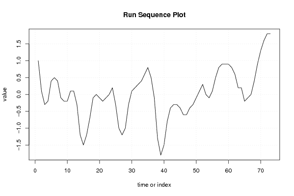
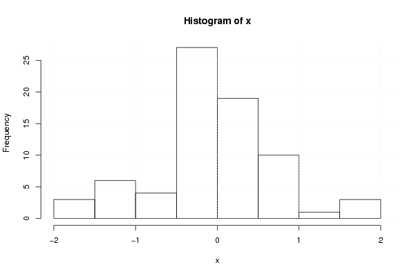
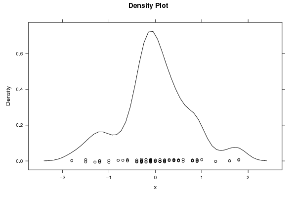
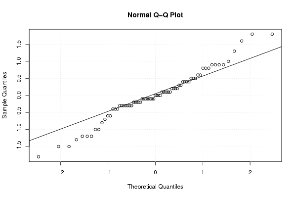
1.00 0.10 -0.30 -0.20 0.40 0.50 0.40 -0.10 -0.20 -0.20 0.10 0.10 -0.30 -1.20 -1.50 -1.20 -0.70 -0.10 0.00 -0.10 -0.20 -0.10 0.00 0.20 -0.30 -1.00 -1.20 -1.00 -0.30 0.10 0.20 0.30 0.40 0.60 0.80 0.50 -0.10 -1.30 -1.80 -1.50 -0.80 -0.40 -0.30 -0.30 -0.40 -0.60 -0.60 -0.40 -0.30 -0.10 0.10 0.30 0.00 -0.10 0.10 0.50 0.80 0.90 0.90 0.90 0.80 0.60 0.20 0.20 -0.20 -0.10 0.00 0.40 0.90 1.30 1.60 1.80 1.80 | |||||||||||||||||||||||||||||||||||||||||||||||||||||
Tables (Output of Computation) | |||||||||||||||||||||||||||||||||||||||||||||||||||||
| |||||||||||||||||||||||||||||||||||||||||||||||||||||
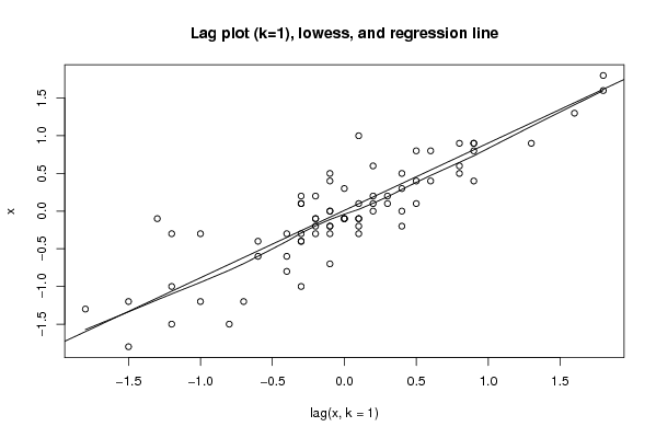
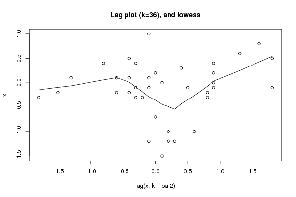
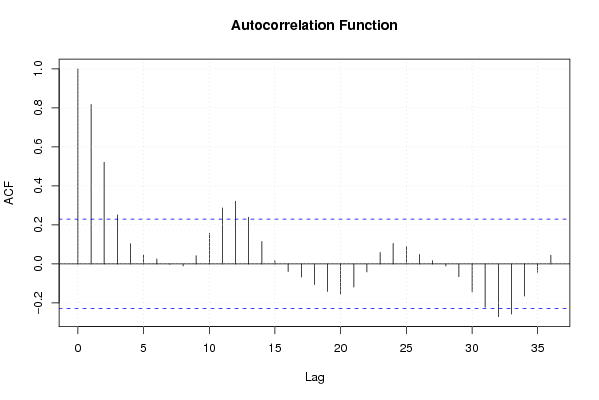
Figures (Output of Computation) | |||||||||||||||||||||||||||||||||||||||||||||||||||||
Input Parameters & R Code | |||||||||||||||||||||||||||||||||||||||||||||||||||||
| Parameters (Session): | |||||||||||||||||||||||||||||||||||||||||||||||||||||
| par1 = 0 ; par2 = 36 ; | |||||||||||||||||||||||||||||||||||||||||||||||||||||
| Parameters (R input): | |||||||||||||||||||||||||||||||||||||||||||||||||||||
| par1 = 0 ; par2 = 36 ; | |||||||||||||||||||||||||||||||||||||||||||||||||||||
| R code (references can be found in the software module): | |||||||||||||||||||||||||||||||||||||||||||||||||||||
par1 <- as.numeric(par1) | |||||||||||||||||||||||||||||||||||||||||||||||||||||