Repository of Reproducible Computations

Free Statistics

of Irreproducible Research!

Author's title

Author

*The author of this computation has been verified*

R Software Module

rwasp_edauni.wasp

Title produced by software

Univariate Explorative Data Analysis

Date of computation

Tue, 20 Oct 2009 11:12:32 -0600

Cite this page as follows

Statistical Computations at FreeStatistics.org, Office for Research Development and Education, URL https://freestatistics.org/blog/index.php?v=date/2009/Oct/20/t1256058801fjncl0xjwyy4iow.htm/, Retrieved Thu, 02 May 2024 20:30:38 +0000

Statistical Computations at FreeStatistics.org, Office for Research Development and Education, URL https://freestatistics.org/blog/index.php?pk=48838, Retrieved Thu, 02 May 2024 20:30:38 +0000

QR Codes:

Paste this QR Code to cite your computation.

Original text written by user:

IsPrivate?

No (this computation is public)

User-defined keywords

Estimated Impact

119

Family? (F = Feedback message, R = changed R code, M = changed R Module, P = changed Parameters, D = changed Data)

-     [Bivariate Data Series] [Bivariate dataset] [2008-01-05 23:51:08] [74be16979710d4c4e7c6647856088456]
F RMPD  [Univariate Explorative Data Analysis] [Colombia Coffee] [2008-01-07 14:21:11] [74be16979710d4c4e7c6647856088456]
F RMPD    [Univariate Data Series] [] [2009-10-14 08:30:28] [74be16979710d4c4e7c6647856088456]
- RMPD      [Central Tendency] [WS3 Part2 Vraag1] [2009-10-18 08:54:29] [42ad1186d39724f834063794eac7cea3]
- RMPD          [Univariate Explorative Data Analysis] [WS3 Part2 Vraag2 TVD] [2009-10-20 17:12:32] [37de18e38c1490dd77c2b362ed87f3bb] [Current]
-                 [Univariate Explorative Data Analysis] [WS3 part 2 vraag2b] [2009-10-21 06:20:38] [f5d341d4bbba73282fc6e80153a6d315] 
-                 [Univariate Explorative Data Analysis] [BDM 8] [2009-10-21 08:37:45] [f5d341d4bbba73282fc6e80153a6d315] 
-                 [Univariate Explorative Data Analysis] [TG 8] [2009-10-21 09:02:09] [a21bac9c8d3d56fdec8be4e719e2c7ed] 

Feedback Forum

Post a new message

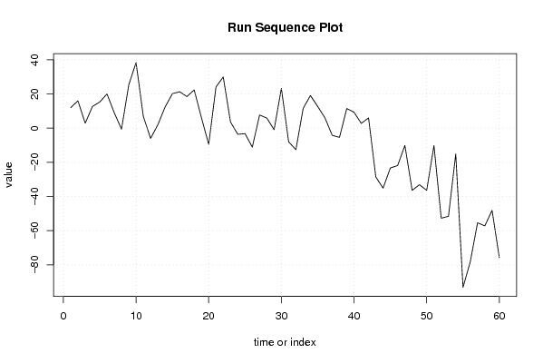
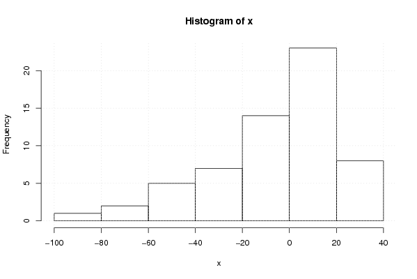
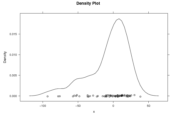
Dataseries X:

Download CSV

Histogram

Boxplots

12
16
2.9
12.7
15.3
20
9
-0.6
25.4
38.4
6.9
-6
2
12.4
20.2
21.3
18.5
22.4
6.1
-9.5
24.1
30
3.6
-3.6
-3.2
-11.1
7.7
5.9
-0.9
23.3
-8
-12.6
11.6
19.1
12.7
6
-4.2
-5.4
11.5
9.3
2.8
6
-28.6
-35.1
-23.3
-21.9
-10.1
-36.4
-33.1
-36.4
-10.2
-52.7
-51.6
-15.1
-93.2
-78.2
-55.4
-57.2
-48.1
-75.9

Summary of computational transaction
Raw Input	view raw input (R code)
Raw Output	view raw output of R engine
Computing time	4 seconds
R Server	'RServer@AstonUniversity' @ vre.aston.ac.uk

\begin{tabular}{lllllllll}
\hline
Summary of computational transaction \tabularnewline
Raw Input & view raw input (R code)  \tabularnewline
Raw Output & view raw output of R engine  \tabularnewline
Computing time & 4 seconds \tabularnewline
R Server & 'RServer@AstonUniversity' @ vre.aston.ac.uk \tabularnewline
\hline
\end{tabular}
%Source: https://freestatistics.org/blog/index.php?pk=48838&T=0

[TABLE]
[ROW][C]Summary of computational transaction[/C][/ROW]
[ROW][C]Raw Input[/C][C]view raw input (R code) [/C][/ROW]
[ROW][C]Raw Output[/C][C]view raw output of R engine [/C][/ROW]
[ROW][C]Computing time[/C][C]4 seconds[/C][/ROW]
[ROW][C]R Server[/C][C]'RServer@AstonUniversity' @ vre.aston.ac.uk[/C][/ROW]
[/TABLE]
Source: https://freestatistics.org/blog/index.php?pk=48838&T=0

Globally Unique Identifier (entire table): ba.freestatistics.org/blog/index.php?pk=48838&T=0

As an alternative you can also use a QR Code:

The GUIDs for individual cells are displayed in the table below:

Summary of computational transaction
Raw Input	view raw input (R code)
Raw Output	view raw output of R engine
Computing time	4 seconds
R Server	'RServer@AstonUniversity' @ vre.aston.ac.uk

Descriptive Statistics
# observations	60
minimum	-93.2
Q1	-16.8
median	2.4
mean	-6.54166666666667
Q3	12.475
maximum	38.4

\begin{tabular}{lllllllll}
\hline
Descriptive Statistics \tabularnewline
# observations & 60 \tabularnewline
minimum & -93.2 \tabularnewline
Q1 & -16.8 \tabularnewline
median & 2.4 \tabularnewline
mean & -6.54166666666667 \tabularnewline
Q3 & 12.475 \tabularnewline
maximum & 38.4 \tabularnewline
\hline
\end{tabular}
%Source: https://freestatistics.org/blog/index.php?pk=48838&T=1

[TABLE]
[ROW][C]Descriptive Statistics[/C][/ROW]
[ROW][C]# observations[/C][C]60[/C][/ROW]
[ROW][C]minimum[/C][C]-93.2[/C][/ROW]
[ROW][C]Q1[/C][C]-16.8[/C][/ROW]
[ROW][C]median[/C][C]2.4[/C][/ROW]
[ROW][C]mean[/C][C]-6.54166666666667[/C][/ROW]
[ROW][C]Q3[/C][C]12.475[/C][/ROW]
[ROW][C]maximum[/C][C]38.4[/C][/ROW]
[/TABLE]
Source: https://freestatistics.org/blog/index.php?pk=48838&T=1

Globally Unique Identifier (entire table): ba.freestatistics.org/blog/index.php?pk=48838&T=1

As an alternative you can also use a QR Code:

The GUIDs for individual cells are displayed in the table below:

Descriptive Statistics
# observations	60
minimum	-93.2
Q1	-16.8
median	2.4
mean	-6.54166666666667
Q3	12.475
maximum	38.4

Figure 1

PNG link

Postscript link

PDF link

Figure 2

PNG link

Postscript link

PDF link

Figure 3

PNG link

Postscript link

PDF link

Figure 4

PNG link

Postscript link

PDF link

Figure 5

PNG link

Postscript link

PDF link

Figure 6

PNG link

Postscript link

PDF link

Figure 7

PNG link

Postscript link

PDF link

Parameters (Session):

par1 = 0 ; par2 = 36 ;

Parameters (R input):

par1 = 0 ; par2 = 36 ;

R code (references can be found in the software module):

par1 <- as.numeric(par1)
par2 <- as.numeric(par2)
x <- as.ts(x)
library(lattice)
bitmap(file='pic1.png')
plot(x,type='l',main='Run Sequence Plot',xlab='time or index',ylab='value')
grid()
dev.off()
bitmap(file='pic2.png')
hist(x)
grid()
dev.off()
bitmap(file='pic3.png')
if (par1 > 0)
{
densityplot(~x,col='black',main=paste('Density Plot   bw = ',par1),bw=par1)
} else {
densityplot(~x,col='black',main='Density Plot')
}
dev.off()
bitmap(file='pic4.png')
qqnorm(x)
qqline(x)
grid()
dev.off()
if (par2 > 0)
{
bitmap(file='lagplot1.png')
dum <- cbind(lag(x,k=1),x)
dum
dum1 <- dum[2:length(x),]
dum1
z <- as.data.frame(dum1)
z
plot(z,main='Lag plot (k=1), lowess, and regression line')
lines(lowess(z))
abline(lm(z))
dev.off()
if (par2 > 1) {
bitmap(file='lagplotpar2.png')
dum <- cbind(lag(x,k=par2),x)
dum
dum1 <- dum[(par2+1):length(x),]
dum1
z <- as.data.frame(dum1)
z
mylagtitle <- 'Lag plot (k='
mylagtitle <- paste(mylagtitle,par2,sep='')
mylagtitle <- paste(mylagtitle,'), and lowess',sep='')
plot(z,main=mylagtitle)
lines(lowess(z))
dev.off()
}
bitmap(file='pic5.png')
acf(x,lag.max=par2,main='Autocorrelation Function')
grid()
dev.off()
}
summary(x)
load(file='createtable')
a<-table.start()
a<-table.row.start(a)
a<-table.element(a,'Descriptive Statistics',2,TRUE)
a<-table.row.end(a)
a<-table.row.start(a)
a<-table.element(a,'# observations',header=TRUE)
a<-table.element(a,length(x))
a<-table.row.end(a)
a<-table.row.start(a)
a<-table.element(a,'minimum',header=TRUE)
a<-table.element(a,min(x))
a<-table.row.end(a)
a<-table.row.start(a)
a<-table.element(a,'Q1',header=TRUE)
a<-table.element(a,quantile(x,0.25))
a<-table.row.end(a)
a<-table.row.start(a)
a<-table.element(a,'median',header=TRUE)
a<-table.element(a,median(x))
a<-table.row.end(a)
a<-table.row.start(a)
a<-table.element(a,'mean',header=TRUE)
a<-table.element(a,mean(x))
a<-table.row.end(a)
a<-table.row.start(a)
a<-table.element(a,'Q3',header=TRUE)
a<-table.element(a,quantile(x,0.75))
a<-table.row.end(a)
a<-table.row.start(a)
a<-table.element(a,'maximum',header=TRUE)
a<-table.element(a,max(x))
a<-table.row.end(a)
a<-table.end(a)
table.save(a,file='mytable.tab')

Free Statistics

Description of Statistical Computation

Tree of Dependent Computations

Dataset

Tables (Output of Computation)

Figures (Output of Computation)

Input Parameters & R Code