\begin{tabular}{lllllllll}
\hline
Summary of computational transaction \tabularnewline
Raw Input & view raw input (R code)  \tabularnewline
Raw Output & view raw output of R engine  \tabularnewline
Computing time & 2 seconds \tabularnewline
R Server & 'Sir Ronald Aylmer Fisher' @ 193.190.124.24 \tabularnewline
\hline
\end{tabular}
%Source: https://freestatistics.org/blog/index.php?pk=47358&T=0
[TABLE]
[ROW][C]Summary of computational transaction[/C][/ROW]
[ROW][C]Raw Input[/C][C]view raw input (R code) [/C][/ROW]
[ROW][C]Raw Output[/C][C]view raw output of R engine [/C][/ROW]
[ROW][C]Computing time[/C][C]2 seconds[/C][/ROW]
[ROW][C]R Server[/C][C]'Sir Ronald Aylmer Fisher' @ 193.190.124.24[/C][/ROW]
[/TABLE]
Source: https://freestatistics.org/blog/index.php?pk=47358&T=0
If you paste this QR Code into your document, anyone with a smartphone or tablet will be able to scan it and view this table in a browser.
If you paste this QR Code into your document, anyone with a smartphone or tablet will be able to scan it and view this table in a browser.
If you paste this QR Code into your document, anyone with a smartphone or tablet will be able to scan it and view this table in a browser.
If you paste this QR Code into your document, anyone with a smartphone or tablet will be able to scan it and view this table in a browser.
If you paste this QR Code into your document, anyone with a smartphone or tablet will be able to scan it and view this table in a browser.
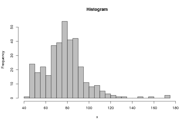
| Frequency Table (Histogram) | | Bins | Midpoint | Abs. Frequency | Rel. Frequency | Cumul. Rel. Freq. | Density | | [40,45[ | 42.5 | 1 | 0.002778 | 0.002778 | 0.000556 | | [45,50[ | 47.5 | 24 | 0.066667 | 0.069444 | 0.013333 | | [50,55[ | 52.5 | 18 | 0.05 | 0.119444 | 0.01 | | [55,60[ | 57.5 | 22 | 0.061111 | 0.180556 | 0.012222 | | [60,65[ | 62.5 | 16 | 0.044444 | 0.225 | 0.008889 | | [65,70[ | 67.5 | 37 | 0.102778 | 0.327778 | 0.020556 | | [70,75[ | 72.5 | 39 | 0.108333 | 0.436111 | 0.021667 | | [75,80[ | 77.5 | 54 | 0.15 | 0.586111 | 0.03 | | [80,85[ | 82.5 | 41 | 0.113889 | 0.7 | 0.022778 | | [85,90[ | 87.5 | 42 | 0.116667 | 0.816667 | 0.023333 | | [90,95[ | 92.5 | 22 | 0.061111 | 0.877778 | 0.012222 | | [95,100[ | 97.5 | 11 | 0.030556 | 0.908333 | 0.006111 | | [100,105[ | 102.5 | 8 | 0.022222 | 0.930556 | 0.004444 | | [105,110[ | 107.5 | 9 | 0.025 | 0.955556 | 0.005 | | [110,115[ | 112.5 | 5 | 0.013889 | 0.969444 | 0.002778 | | [115,120[ | 117.5 | 3 | 0.008333 | 0.977778 | 0.001667 | | [120,125[ | 122.5 | 2 | 0.005556 | 0.983333 | 0.001111 | | [125,130[ | 127.5 | 1 | 0.002778 | 0.986111 | 0.000556 | | [130,135[ | 132.5 | 1 | 0.002778 | 0.988889 | 0.000556 | | [135,140[ | 137.5 | 0 | 0 | 0.988889 | 0 | | [140,145[ | 142.5 | 0 | 0 | 0.988889 | 0 | | [145,150[ | 147.5 | 1 | 0.002778 | 0.991667 | 0.000556 | | [150,155[ | 152.5 | 0 | 0 | 0.991667 | 0 | | [155,160[ | 157.5 | 1 | 0.002778 | 0.994444 | 0.000556 | | [160,165[ | 162.5 | 0 | 0 | 0.994444 | 0 | | [165,170[ | 167.5 | 0 | 0 | 0.994444 | 0 | | [170,175] | 172.5 | 2 | 0.005556 | 1 | 0.001111 |
\begin{tabular}{lllllllll}
\hline
Frequency Table (Histogram) \tabularnewline
Bins & Midpoint & Abs. Frequency & Rel. Frequency & Cumul. Rel. Freq. & Density \tabularnewline
[40,45[ & 42.5 & 1 & 0.002778 & 0.002778 & 0.000556 \tabularnewline
[45,50[ & 47.5 & 24 & 0.066667 & 0.069444 & 0.013333 \tabularnewline
[50,55[ & 52.5 & 18 & 0.05 & 0.119444 & 0.01 \tabularnewline
[55,60[ & 57.5 & 22 & 0.061111 & 0.180556 & 0.012222 \tabularnewline
[60,65[ & 62.5 & 16 & 0.044444 & 0.225 & 0.008889 \tabularnewline
[65,70[ & 67.5 & 37 & 0.102778 & 0.327778 & 0.020556 \tabularnewline
[70,75[ & 72.5 & 39 & 0.108333 & 0.436111 & 0.021667 \tabularnewline
[75,80[ & 77.5 & 54 & 0.15 & 0.586111 & 0.03 \tabularnewline
[80,85[ & 82.5 & 41 & 0.113889 & 0.7 & 0.022778 \tabularnewline
[85,90[ & 87.5 & 42 & 0.116667 & 0.816667 & 0.023333 \tabularnewline
[90,95[ & 92.5 & 22 & 0.061111 & 0.877778 & 0.012222 \tabularnewline
[95,100[ & 97.5 & 11 & 0.030556 & 0.908333 & 0.006111 \tabularnewline
[100,105[ & 102.5 & 8 & 0.022222 & 0.930556 & 0.004444 \tabularnewline
[105,110[ & 107.5 & 9 & 0.025 & 0.955556 & 0.005 \tabularnewline
[110,115[ & 112.5 & 5 & 0.013889 & 0.969444 & 0.002778 \tabularnewline
[115,120[ & 117.5 & 3 & 0.008333 & 0.977778 & 0.001667 \tabularnewline
[120,125[ & 122.5 & 2 & 0.005556 & 0.983333 & 0.001111 \tabularnewline
[125,130[ & 127.5 & 1 & 0.002778 & 0.986111 & 0.000556 \tabularnewline
[130,135[ & 132.5 & 1 & 0.002778 & 0.988889 & 0.000556 \tabularnewline
[135,140[ & 137.5 & 0 & 0 & 0.988889 & 0 \tabularnewline
[140,145[ & 142.5 & 0 & 0 & 0.988889 & 0 \tabularnewline
[145,150[ & 147.5 & 1 & 0.002778 & 0.991667 & 0.000556 \tabularnewline
[150,155[ & 152.5 & 0 & 0 & 0.991667 & 0 \tabularnewline
[155,160[ & 157.5 & 1 & 0.002778 & 0.994444 & 0.000556 \tabularnewline
[160,165[ & 162.5 & 0 & 0 & 0.994444 & 0 \tabularnewline
[165,170[ & 167.5 & 0 & 0 & 0.994444 & 0 \tabularnewline
[170,175] & 172.5 & 2 & 0.005556 & 1 & 0.001111 \tabularnewline
\hline
\end{tabular}
%Source: https://freestatistics.org/blog/index.php?pk=47358&T=1
[TABLE]
[ROW][C]Frequency Table (Histogram)[/C][/ROW]
[ROW][C]Bins[/C][C]Midpoint[/C][C]Abs. Frequency[/C][C]Rel. Frequency[/C][C]Cumul. Rel. Freq.[/C][C]Density[/C][/ROW]
[ROW][C][40,45[[/C][C]42.5[/C][C]1[/C][C]0.002778[/C][C]0.002778[/C][C]0.000556[/C][/ROW]
[ROW][C][45,50[[/C][C]47.5[/C][C]24[/C][C]0.066667[/C][C]0.069444[/C][C]0.013333[/C][/ROW]
[ROW][C][50,55[[/C][C]52.5[/C][C]18[/C][C]0.05[/C][C]0.119444[/C][C]0.01[/C][/ROW]
[ROW][C][55,60[[/C][C]57.5[/C][C]22[/C][C]0.061111[/C][C]0.180556[/C][C]0.012222[/C][/ROW]
[ROW][C][60,65[[/C][C]62.5[/C][C]16[/C][C]0.044444[/C][C]0.225[/C][C]0.008889[/C][/ROW]
[ROW][C][65,70[[/C][C]67.5[/C][C]37[/C][C]0.102778[/C][C]0.327778[/C][C]0.020556[/C][/ROW]
[ROW][C][70,75[[/C][C]72.5[/C][C]39[/C][C]0.108333[/C][C]0.436111[/C][C]0.021667[/C][/ROW]
[ROW][C][75,80[[/C][C]77.5[/C][C]54[/C][C]0.15[/C][C]0.586111[/C][C]0.03[/C][/ROW]
[ROW][C][80,85[[/C][C]82.5[/C][C]41[/C][C]0.113889[/C][C]0.7[/C][C]0.022778[/C][/ROW]
[ROW][C][85,90[[/C][C]87.5[/C][C]42[/C][C]0.116667[/C][C]0.816667[/C][C]0.023333[/C][/ROW]
[ROW][C][90,95[[/C][C]92.5[/C][C]22[/C][C]0.061111[/C][C]0.877778[/C][C]0.012222[/C][/ROW]
[ROW][C][95,100[[/C][C]97.5[/C][C]11[/C][C]0.030556[/C][C]0.908333[/C][C]0.006111[/C][/ROW]
[ROW][C][100,105[[/C][C]102.5[/C][C]8[/C][C]0.022222[/C][C]0.930556[/C][C]0.004444[/C][/ROW]
[ROW][C][105,110[[/C][C]107.5[/C][C]9[/C][C]0.025[/C][C]0.955556[/C][C]0.005[/C][/ROW]
[ROW][C][110,115[[/C][C]112.5[/C][C]5[/C][C]0.013889[/C][C]0.969444[/C][C]0.002778[/C][/ROW]
[ROW][C][115,120[[/C][C]117.5[/C][C]3[/C][C]0.008333[/C][C]0.977778[/C][C]0.001667[/C][/ROW]
[ROW][C][120,125[[/C][C]122.5[/C][C]2[/C][C]0.005556[/C][C]0.983333[/C][C]0.001111[/C][/ROW]
[ROW][C][125,130[[/C][C]127.5[/C][C]1[/C][C]0.002778[/C][C]0.986111[/C][C]0.000556[/C][/ROW]
[ROW][C][130,135[[/C][C]132.5[/C][C]1[/C][C]0.002778[/C][C]0.988889[/C][C]0.000556[/C][/ROW]
[ROW][C][135,140[[/C][C]137.5[/C][C]0[/C][C]0[/C][C]0.988889[/C][C]0[/C][/ROW]
[ROW][C][140,145[[/C][C]142.5[/C][C]0[/C][C]0[/C][C]0.988889[/C][C]0[/C][/ROW]
[ROW][C][145,150[[/C][C]147.5[/C][C]1[/C][C]0.002778[/C][C]0.991667[/C][C]0.000556[/C][/ROW]
[ROW][C][150,155[[/C][C]152.5[/C][C]0[/C][C]0[/C][C]0.991667[/C][C]0[/C][/ROW]
[ROW][C][155,160[[/C][C]157.5[/C][C]1[/C][C]0.002778[/C][C]0.994444[/C][C]0.000556[/C][/ROW]
[ROW][C][160,165[[/C][C]162.5[/C][C]0[/C][C]0[/C][C]0.994444[/C][C]0[/C][/ROW]
[ROW][C][165,170[[/C][C]167.5[/C][C]0[/C][C]0[/C][C]0.994444[/C][C]0[/C][/ROW]
[ROW][C][170,175][/C][C]172.5[/C][C]2[/C][C]0.005556[/C][C]1[/C][C]0.001111[/C][/ROW]
[/TABLE]
Source: https://freestatistics.org/blog/index.php?pk=47358&T=1
Globally Unique Identifier (entire table): ba.freestatistics.org/blog/index.php?pk=47358&T=1
As an alternative you can also use a QR Code:
The GUIDs for individual cells are displayed in the table below:
| Frequency Table (Histogram) | | Bins | Midpoint | Abs. Frequency | Rel. Frequency | Cumul. Rel. Freq. | Density | | [40,45[ | 42.5 | 1 | 0.002778 | 0.002778 | 0.000556 | | [45,50[ | 47.5 | 24 | 0.066667 | 0.069444 | 0.013333 | | [50,55[ | 52.5 | 18 | 0.05 | 0.119444 | 0.01 | | [55,60[ | 57.5 | 22 | 0.061111 | 0.180556 | 0.012222 | | [60,65[ | 62.5 | 16 | 0.044444 | 0.225 | 0.008889 | | [65,70[ | 67.5 | 37 | 0.102778 | 0.327778 | 0.020556 | | [70,75[ | 72.5 | 39 | 0.108333 | 0.436111 | 0.021667 | | [75,80[ | 77.5 | 54 | 0.15 | 0.586111 | 0.03 | | [80,85[ | 82.5 | 41 | 0.113889 | 0.7 | 0.022778 | | [85,90[ | 87.5 | 42 | 0.116667 | 0.816667 | 0.023333 | | [90,95[ | 92.5 | 22 | 0.061111 | 0.877778 | 0.012222 | | [95,100[ | 97.5 | 11 | 0.030556 | 0.908333 | 0.006111 | | [100,105[ | 102.5 | 8 | 0.022222 | 0.930556 | 0.004444 | | [105,110[ | 107.5 | 9 | 0.025 | 0.955556 | 0.005 | | [110,115[ | 112.5 | 5 | 0.013889 | 0.969444 | 0.002778 | | [115,120[ | 117.5 | 3 | 0.008333 | 0.977778 | 0.001667 | | [120,125[ | 122.5 | 2 | 0.005556 | 0.983333 | 0.001111 | | [125,130[ | 127.5 | 1 | 0.002778 | 0.986111 | 0.000556 | | [130,135[ | 132.5 | 1 | 0.002778 | 0.988889 | 0.000556 | | [135,140[ | 137.5 | 0 | 0 | 0.988889 | 0 | | [140,145[ | 142.5 | 0 | 0 | 0.988889 | 0 | | [145,150[ | 147.5 | 1 | 0.002778 | 0.991667 | 0.000556 | | [150,155[ | 152.5 | 0 | 0 | 0.991667 | 0 | | [155,160[ | 157.5 | 1 | 0.002778 | 0.994444 | 0.000556 | | [160,165[ | 162.5 | 0 | 0 | 0.994444 | 0 | | [165,170[ | 167.5 | 0 | 0 | 0.994444 | 0 | | [170,175] | 172.5 | 2 | 0.005556 | 1 | 0.001111 |
If you paste this QR Code into your document, anyone with a smartphone or tablet will be able to scan it and view this table in a browser.
If you paste this QR Code into your document, anyone with a smartphone or tablet will be able to scan it and view this table in a browser.
If you paste this QR Code into your document, anyone with a smartphone or tablet will be able to scan it and view this table in a browser.
If you paste this QR Code into your document, anyone with a smartphone or tablet will be able to scan it and view this table in a browser.
If you paste this QR Code into your document, anyone with a smartphone or tablet will be able to scan it and view this table in a browser.
|