Free Statistics
of Irreproducible Research!
Description of Statistical Computation | |||||||||||||||||||||||||||||||||||||||||||||||||||||||||||||||||||||||||
|---|---|---|---|---|---|---|---|---|---|---|---|---|---|---|---|---|---|---|---|---|---|---|---|---|---|---|---|---|---|---|---|---|---|---|---|---|---|---|---|---|---|---|---|---|---|---|---|---|---|---|---|---|---|---|---|---|---|---|---|---|---|---|---|---|---|---|---|---|---|---|---|---|---|
| Author's title | |||||||||||||||||||||||||||||||||||||||||||||||||||||||||||||||||||||||||
| Author | *The author of this computation has been verified* | ||||||||||||||||||||||||||||||||||||||||||||||||||||||||||||||||||||||||
| R Software Module | rwasp_babies.wasp | ||||||||||||||||||||||||||||||||||||||||||||||||||||||||||||||||||||||||
| Title produced by software | Exercise 1.13 | ||||||||||||||||||||||||||||||||||||||||||||||||||||||||||||||||||||||||
| Date of computation | Wed, 07 Oct 2009 14:34:03 -0600 | ||||||||||||||||||||||||||||||||||||||||||||||||||||||||||||||||||||||||
| Cite this page as follows | Statistical Computations at FreeStatistics.org, Office for Research Development and Education, URL https://freestatistics.org/blog/index.php?v=date/2009/Oct/07/t1254947804eae9pdavu9vh340.htm/, Retrieved Sun, 28 Apr 2024 18:09:22 +0000 | ||||||||||||||||||||||||||||||||||||||||||||||||||||||||||||||||||||||||
| Statistical Computations at FreeStatistics.org, Office for Research Development and Education, URL https://freestatistics.org/blog/index.php?pk=44795, Retrieved Sun, 28 Apr 2024 18:09:22 +0000 | |||||||||||||||||||||||||||||||||||||||||||||||||||||||||||||||||||||||||
| QR Codes: | |||||||||||||||||||||||||||||||||||||||||||||||||||||||||||||||||||||||||
|
| |||||||||||||||||||||||||||||||||||||||||||||||||||||||||||||||||||||||||
| Original text written by user: | |||||||||||||||||||||||||||||||||||||||||||||||||||||||||||||||||||||||||
| IsPrivate? | No (this computation is public) | ||||||||||||||||||||||||||||||||||||||||||||||||||||||||||||||||||||||||
| User-defined keywords | |||||||||||||||||||||||||||||||||||||||||||||||||||||||||||||||||||||||||
| Estimated Impact | 195 | ||||||||||||||||||||||||||||||||||||||||||||||||||||||||||||||||||||||||
Tree of Dependent Computations | |||||||||||||||||||||||||||||||||||||||||||||||||||||||||||||||||||||||||
| Family? (F = Feedback message, R = changed R code, M = changed R Module, P = changed Parameters, D = changed Data) | |||||||||||||||||||||||||||||||||||||||||||||||||||||||||||||||||||||||||
| - [Exercise 1.13] [Ex. 1.13 Babies c...] [2009-10-07 19:52:56] [62d80b0d35658f72f0b015f194fffbd1] - P [Exercise 1.13] [Ex. 1.13 Babies c...] [2009-10-07 20:14:54] [62d80b0d35658f72f0b015f194fffbd1] - R [Exercise 1.13] [Ex. 1.13 Babies c...] [2009-10-07 20:34:03] [fe4830fadb816e957b418931db9ed257] [Current] - R [Exercise 1.13] [Correction on rev...] [2009-10-12 18:23:15] [df1349bc077b4746949c1672214183f7] F RMPD [Univariate Data Series] [1e grafiek] [2009-10-12 19:18:44] [df1349bc077b4746949c1672214183f7] F RMPD [Univariate Data Series] [2e grafiek, indus...] [2009-10-12 20:19:32] [df1349bc077b4746949c1672214183f7] - RMPD [Univariate Data Series] [3e grafiek] [2009-10-12 22:01:20] [df1349bc077b4746949c1672214183f7] - RMPD [Univariate Data Series] [3e grafiek] [2009-10-12 22:09:25] [df1349bc077b4746949c1672214183f7] F RMPD [Univariate Data Series] [3e grafiek] [2009-10-12 22:14:27] [df1349bc077b4746949c1672214183f7] - PD [Univariate Data Series] [Y[t] - X[t] = c +...] [2009-10-20 19:10:29] [df1349bc077b4746949c1672214183f7] - PD [Univariate Data Series] [Y[t] / X[t] = c +...] [2009-10-20 19:15:17] [df1349bc077b4746949c1672214183f7] - RM D [Central Tendency] [Central Tendency ...] [2009-10-20 19:21:07] [df1349bc077b4746949c1672214183f7] - RM [Harrell-Davis Quantiles] [Harrel Davis 95% ...] [2009-10-20 19:29:53] [df1349bc077b4746949c1672214183f7] - RM [Percentiles] [Percentiles 80% P...] [2009-10-20 19:34:55] [df1349bc077b4746949c1672214183f7] - PD [Central Tendency] [workshop 3 part 3] [2009-10-21 17:22:50] [af8eb90b4bf1bcfcc4325c143dbee260] F RMPD [Univariate Data Series] [4e grafiek] [2009-10-12 22:29:21] [df1349bc077b4746949c1672214183f7] | |||||||||||||||||||||||||||||||||||||||||||||||||||||||||||||||||||||||||
| Feedback Forum | |||||||||||||||||||||||||||||||||||||||||||||||||||||||||||||||||||||||||
Post a new message | |||||||||||||||||||||||||||||||||||||||||||||||||||||||||||||||||||||||||
Dataset | |||||||||||||||||||||||||||||||||||||||||||||||||||||||||||||||||||||||||
Tables (Output of Computation) | |||||||||||||||||||||||||||||||||||||||||||||||||||||||||||||||||||||||||
| |||||||||||||||||||||||||||||||||||||||||||||||||||||||||||||||||||||||||
Figures (Output of Computation) | |||||||||||||||||||||||||||||||||||||||||||||||||||||||||||||||||||||||||
Input Parameters & R Code | |||||||||||||||||||||||||||||||||||||||||||||||||||||||||||||||||||||||||
| Parameters (Session): | |||||||||||||||||||||||||||||||||||||||||||||||||||||||||||||||||||||||||
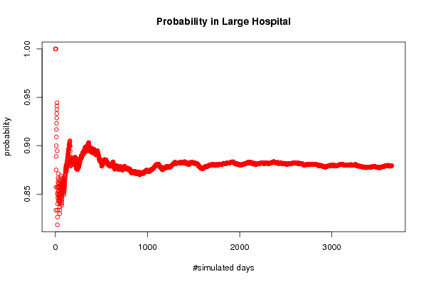
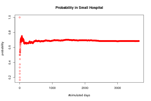
| par1 = 3650 ; par2 = 45 ; par3 = 15 ; par4 = 0.6 ; | |||||||||||||||||||||||||||||||||||||||||||||||||||||||||||||||||||||||||
| Parameters (R input): | |||||||||||||||||||||||||||||||||||||||||||||||||||||||||||||||||||||||||
| par1 = 3650 ; par2 = 45 ; par3 = 15 ; par4 = 0.6 ; | |||||||||||||||||||||||||||||||||||||||||||||||||||||||||||||||||||||||||
| R code (references can be found in the software module): | |||||||||||||||||||||||||||||||||||||||||||||||||||||||||||||||||||||||||
par1 <- as.numeric(par1) | |||||||||||||||||||||||||||||||||||||||||||||||||||||||||||||||||||||||||