Repository of Reproducible Computations

Free Statistics

of Irreproducible Research!

Author's title

Author

*The author of this computation has been verified*

R Software Module

rwasp_autocorrelation.wasp

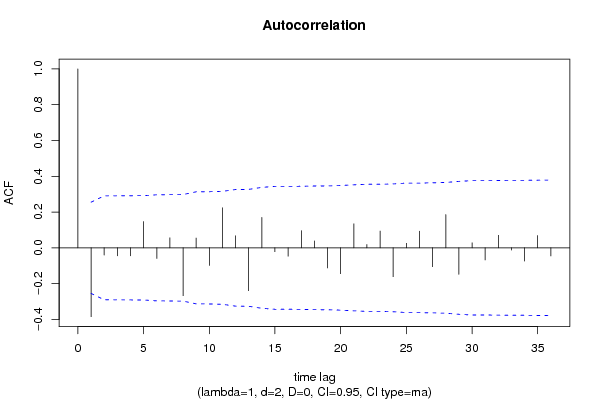
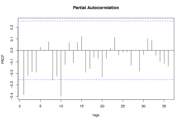
Title produced by software

(Partial) Autocorrelation Function

Date of computation

Sun, 29 Nov 2009 09:25:50 -0700

Cite this page as follows

Statistical Computations at FreeStatistics.org, Office for Research Development and Education, URL https://freestatistics.org/blog/index.php?v=date/2009/Nov/29/t12595120072dl6vjz8r33ef1n.htm/, Retrieved Thu, 25 Apr 2024 10:45:37 +0000

Statistical Computations at FreeStatistics.org, Office for Research Development and Education, URL https://freestatistics.org/blog/index.php?pk=61657, Retrieved Thu, 25 Apr 2024 10:45:37 +0000

QR Codes:

Paste this QR Code to cite your computation.

Original text written by user:

IsPrivate?

No (this computation is public)

User-defined keywords

Estimated Impact

126

Family? (F = Feedback message, R = changed R code, M = changed R Module, P = changed Parameters, D = changed Data)

-     [Univariate Explorative Data Analysis] [Run Sequence gebo...] [2008-12-12 13:32:37] [76963dc1903f0f612b6153510a3818cf]
- R  D  [Univariate Explorative Data Analysis] [Run Sequence gebo...] [2008-12-17 12:14:40] [76963dc1903f0f612b6153510a3818cf]
-         [Univariate Explorative Data Analysis] [Run Sequence Plot...] [2008-12-22 18:19:51] [1ce0d16c8f4225c977b42c8fa93bc163]
- RMP       [(Partial) Autocorrelation Function] [Identifying Integ...] [2009-11-22 12:16:10] [b98453cac15ba1066b407e146608df68]
-    D        [(Partial) Autocorrelation Function] [WS8.2] [2009-11-25 18:11:35] [626f1d98f4a7f05bcb9f17666b672c60]
-    D          [(Partial) Autocorrelation Function] [workshop 8] [2009-11-28 08:51:25] [4fe1472705bb0a32f118ba3ca90ffa8e]
- R P               [(Partial) Autocorrelation Function] [Workshop8 Review ...] [2009-11-29 16:25:50] [5ed0eef5d4509bbfdac0ae6d87f3b4bf] [Current]

Feedback Forum

Post a new message

Dataseries X:

Download CSV

Histogram

Boxplots

Summary of computational transaction
Raw Input	view raw input (R code)
Raw Output	view raw output of R engine
Computing time	1 seconds
R Server	'Gwilym Jenkins' @ 72.249.127.135

\begin{tabular}{lllllllll}
\hline
Summary of computational transaction \tabularnewline
Raw Input & view raw input (R code)  \tabularnewline
Raw Output & view raw output of R engine  \tabularnewline
Computing time & 1 seconds \tabularnewline
R Server & 'Gwilym Jenkins' @ 72.249.127.135 \tabularnewline
\hline
\end{tabular}
%Source: https://freestatistics.org/blog/index.php?pk=61657&T=0

[TABLE]
[ROW][C]Summary of computational transaction[/C][/ROW]
[ROW][C]Raw Input[/C][C]view raw input (R code) [/C][/ROW]
[ROW][C]Raw Output[/C][C]view raw output of R engine [/C][/ROW]
[ROW][C]Computing time[/C][C]1 seconds[/C][/ROW]
[ROW][C]R Server[/C][C]'Gwilym Jenkins' @ 72.249.127.135[/C][/ROW]
[/TABLE]
Source: https://freestatistics.org/blog/index.php?pk=61657&T=0

Globally Unique Identifier (entire table): ba.freestatistics.org/blog/index.php?pk=61657&T=0

As an alternative you can also use a QR Code:

The GUIDs for individual cells are displayed in the table below:

Summary of computational transaction
Raw Input	view raw input (R code)
Raw Output	view raw output of R engine
Computing time	1 seconds
R Server	'Gwilym Jenkins' @ 72.249.127.135

Autocorrelation Function
Time lag k	ACF(k)	T-STAT	P-value
1	-0.384754	-2.9553	0.002241
2	-0.040646	-0.3122	0.377993
3	-0.044529	-0.342	0.36677
4	-0.044338	-0.3406	0.36732
5	0.146971	1.1289	0.131754
6	-0.059001	-0.4532	0.326036
7	0.056172	0.4315	0.333852
8	-0.267648	-2.0558	0.022116
9	0.05433	0.4173	0.33898
10	-0.098231	-0.7545	0.226766
11	0.22397	1.7203	0.045305
12	0.067325	0.5171	0.303499
13	-0.239457	-1.8393	0.035452
14	0.170216	1.3075	0.098066
15	-0.021373	-0.1642	0.435079
16	-0.046856	-0.3599	0.3601
17	0.095927	0.7368	0.232073
18	0.03857	0.2963	0.384035
19	-0.112103	-0.8611	0.196339
20	-0.144606	-1.1107	0.135593
21	0.134526	1.0333	0.152838
22	0.018294	0.1405	0.444364
23	0.093539	0.7185	0.237647
24	-0.161161	-1.2379	0.110329
25	0.025365	0.1948	0.423097
26	0.092871	0.7134	0.239219
27	-0.105637	-0.8114	0.210195
28	0.185662	1.4261	0.079555
29	-0.148195	-1.1383	0.129796
30	0.028055	0.2155	0.415063
31	-0.067895	-0.5215	0.30198
32	0.07002	0.5378	0.296358
33	-0.012348	-0.0948	0.46238
34	-0.074044	-0.5687	0.285844
35	0.068623	0.5271	0.30005
36	-0.045666	-0.3508	0.363505

\begin{tabular}{lllllllll}
\hline
Autocorrelation Function \tabularnewline
Time lag k & ACF(k) & T-STAT & P-value \tabularnewline
1 & -0.384754 & -2.9553 & 0.002241 \tabularnewline
2 & -0.040646 & -0.3122 & 0.377993 \tabularnewline
3 & -0.044529 & -0.342 & 0.36677 \tabularnewline
4 & -0.044338 & -0.3406 & 0.36732 \tabularnewline
5 & 0.146971 & 1.1289 & 0.131754 \tabularnewline
6 & -0.059001 & -0.4532 & 0.326036 \tabularnewline
7 & 0.056172 & 0.4315 & 0.333852 \tabularnewline
8 & -0.267648 & -2.0558 & 0.022116 \tabularnewline
9 & 0.05433 & 0.4173 & 0.33898 \tabularnewline
10 & -0.098231 & -0.7545 & 0.226766 \tabularnewline
11 & 0.22397 & 1.7203 & 0.045305 \tabularnewline
12 & 0.067325 & 0.5171 & 0.303499 \tabularnewline
13 & -0.239457 & -1.8393 & 0.035452 \tabularnewline
14 & 0.170216 & 1.3075 & 0.098066 \tabularnewline
15 & -0.021373 & -0.1642 & 0.435079 \tabularnewline
16 & -0.046856 & -0.3599 & 0.3601 \tabularnewline
17 & 0.095927 & 0.7368 & 0.232073 \tabularnewline
18 & 0.03857 & 0.2963 & 0.384035 \tabularnewline
19 & -0.112103 & -0.8611 & 0.196339 \tabularnewline
20 & -0.144606 & -1.1107 & 0.135593 \tabularnewline
21 & 0.134526 & 1.0333 & 0.152838 \tabularnewline
22 & 0.018294 & 0.1405 & 0.444364 \tabularnewline
23 & 0.093539 & 0.7185 & 0.237647 \tabularnewline
24 & -0.161161 & -1.2379 & 0.110329 \tabularnewline
25 & 0.025365 & 0.1948 & 0.423097 \tabularnewline
26 & 0.092871 & 0.7134 & 0.239219 \tabularnewline
27 & -0.105637 & -0.8114 & 0.210195 \tabularnewline
28 & 0.185662 & 1.4261 & 0.079555 \tabularnewline
29 & -0.148195 & -1.1383 & 0.129796 \tabularnewline
30 & 0.028055 & 0.2155 & 0.415063 \tabularnewline
31 & -0.067895 & -0.5215 & 0.30198 \tabularnewline
32 & 0.07002 & 0.5378 & 0.296358 \tabularnewline
33 & -0.012348 & -0.0948 & 0.46238 \tabularnewline
34 & -0.074044 & -0.5687 & 0.285844 \tabularnewline
35 & 0.068623 & 0.5271 & 0.30005 \tabularnewline
36 & -0.045666 & -0.3508 & 0.363505 \tabularnewline
\hline
\end{tabular}
%Source: https://freestatistics.org/blog/index.php?pk=61657&T=1

[TABLE]
[ROW][C]Autocorrelation Function[/C][/ROW]
[ROW][C]Time lag k[/C][C]ACF(k)[/C][C]T-STAT[/C][C]P-value[/C][/ROW]
[ROW][C]1[/C][C]-0.384754[/C][C]-2.9553[/C][C]0.002241[/C][/ROW]
[ROW][C]2[/C][C]-0.040646[/C][C]-0.3122[/C][C]0.377993[/C][/ROW]
[ROW][C]3[/C][C]-0.044529[/C][C]-0.342[/C][C]0.36677[/C][/ROW]
[ROW][C]4[/C][C]-0.044338[/C][C]-0.3406[/C][C]0.36732[/C][/ROW]
[ROW][C]5[/C][C]0.146971[/C][C]1.1289[/C][C]0.131754[/C][/ROW]
[ROW][C]6[/C][C]-0.059001[/C][C]-0.4532[/C][C]0.326036[/C][/ROW]
[ROW][C]7[/C][C]0.056172[/C][C]0.4315[/C][C]0.333852[/C][/ROW]
[ROW][C]8[/C][C]-0.267648[/C][C]-2.0558[/C][C]0.022116[/C][/ROW]
[ROW][C]9[/C][C]0.05433[/C][C]0.4173[/C][C]0.33898[/C][/ROW]
[ROW][C]10[/C][C]-0.098231[/C][C]-0.7545[/C][C]0.226766[/C][/ROW]
[ROW][C]11[/C][C]0.22397[/C][C]1.7203[/C][C]0.045305[/C][/ROW]
[ROW][C]12[/C][C]0.067325[/C][C]0.5171[/C][C]0.303499[/C][/ROW]
[ROW][C]13[/C][C]-0.239457[/C][C]-1.8393[/C][C]0.035452[/C][/ROW]
[ROW][C]14[/C][C]0.170216[/C][C]1.3075[/C][C]0.098066[/C][/ROW]
[ROW][C]15[/C][C]-0.021373[/C][C]-0.1642[/C][C]0.435079[/C][/ROW]
[ROW][C]16[/C][C]-0.046856[/C][C]-0.3599[/C][C]0.3601[/C][/ROW]
[ROW][C]17[/C][C]0.095927[/C][C]0.7368[/C][C]0.232073[/C][/ROW]
[ROW][C]18[/C][C]0.03857[/C][C]0.2963[/C][C]0.384035[/C][/ROW]
[ROW][C]19[/C][C]-0.112103[/C][C]-0.8611[/C][C]0.196339[/C][/ROW]
[ROW][C]20[/C][C]-0.144606[/C][C]-1.1107[/C][C]0.135593[/C][/ROW]
[ROW][C]21[/C][C]0.134526[/C][C]1.0333[/C][C]0.152838[/C][/ROW]
[ROW][C]22[/C][C]0.018294[/C][C]0.1405[/C][C]0.444364[/C][/ROW]
[ROW][C]23[/C][C]0.093539[/C][C]0.7185[/C][C]0.237647[/C][/ROW]
[ROW][C]24[/C][C]-0.161161[/C][C]-1.2379[/C][C]0.110329[/C][/ROW]
[ROW][C]25[/C][C]0.025365[/C][C]0.1948[/C][C]0.423097[/C][/ROW]
[ROW][C]26[/C][C]0.092871[/C][C]0.7134[/C][C]0.239219[/C][/ROW]
[ROW][C]27[/C][C]-0.105637[/C][C]-0.8114[/C][C]0.210195[/C][/ROW]
[ROW][C]28[/C][C]0.185662[/C][C]1.4261[/C][C]0.079555[/C][/ROW]
[ROW][C]29[/C][C]-0.148195[/C][C]-1.1383[/C][C]0.129796[/C][/ROW]
[ROW][C]30[/C][C]0.028055[/C][C]0.2155[/C][C]0.415063[/C][/ROW]
[ROW][C]31[/C][C]-0.067895[/C][C]-0.5215[/C][C]0.30198[/C][/ROW]
[ROW][C]32[/C][C]0.07002[/C][C]0.5378[/C][C]0.296358[/C][/ROW]
[ROW][C]33[/C][C]-0.012348[/C][C]-0.0948[/C][C]0.46238[/C][/ROW]
[ROW][C]34[/C][C]-0.074044[/C][C]-0.5687[/C][C]0.285844[/C][/ROW]
[ROW][C]35[/C][C]0.068623[/C][C]0.5271[/C][C]0.30005[/C][/ROW]
[ROW][C]36[/C][C]-0.045666[/C][C]-0.3508[/C][C]0.363505[/C][/ROW]
[/TABLE]
Source: https://freestatistics.org/blog/index.php?pk=61657&T=1

Globally Unique Identifier (entire table): ba.freestatistics.org/blog/index.php?pk=61657&T=1

As an alternative you can also use a QR Code:

The GUIDs for individual cells are displayed in the table below:

Autocorrelation Function
Time lag k	ACF(k)	T-STAT	P-value
1	-0.384754	-2.9553	0.002241
2	-0.040646	-0.3122	0.377993
3	-0.044529	-0.342	0.36677
4	-0.044338	-0.3406	0.36732
5	0.146971	1.1289	0.131754
6	-0.059001	-0.4532	0.326036
7	0.056172	0.4315	0.333852
8	-0.267648	-2.0558	0.022116
9	0.05433	0.4173	0.33898
10	-0.098231	-0.7545	0.226766
11	0.22397	1.7203	0.045305
12	0.067325	0.5171	0.303499
13	-0.239457	-1.8393	0.035452
14	0.170216	1.3075	0.098066
15	-0.021373	-0.1642	0.435079
16	-0.046856	-0.3599	0.3601
17	0.095927	0.7368	0.232073
18	0.03857	0.2963	0.384035
19	-0.112103	-0.8611	0.196339
20	-0.144606	-1.1107	0.135593
21	0.134526	1.0333	0.152838
22	0.018294	0.1405	0.444364
23	0.093539	0.7185	0.237647
24	-0.161161	-1.2379	0.110329
25	0.025365	0.1948	0.423097
26	0.092871	0.7134	0.239219
27	-0.105637	-0.8114	0.210195
28	0.185662	1.4261	0.079555
29	-0.148195	-1.1383	0.129796
30	0.028055	0.2155	0.415063
31	-0.067895	-0.5215	0.30198
32	0.07002	0.5378	0.296358
33	-0.012348	-0.0948	0.46238
34	-0.074044	-0.5687	0.285844
35	0.068623	0.5271	0.30005
36	-0.045666	-0.3508	0.363505

Partial Autocorrelation Function
Time lag k	PACF(k)	T-STAT	P-value
1	-0.384754	-2.9553	0.002241
2	-0.221466	-1.7011	0.047094
3	-0.183714	-1.4111	0.081728
4	-0.191959	-1.4745	0.072836
5	0.028012	0.2152	0.415192
6	-0.005264	-0.0404	0.483942
7	0.074511	0.5723	0.284637
8	-0.26044	-2.0005	0.025029
9	-0.224268	-1.7226	0.045096
10	-0.402315	-3.0902	0.001525
11	-0.123437	-0.9481	0.173463
12	0.068275	0.5244	0.300971
13	-0.107915	-0.8289	0.205248
14	0.07115	0.5465	0.293387
15	0.12193	0.9366	0.1764
16	-0.191015	-1.4672	0.073815
17	-0.160292	-1.2312	0.111561
18	-0.05827	-0.4476	0.328048
19	-0.071851	-0.5519	0.291551
20	-0.233493	-1.7935	0.03901
21	-0.071559	-0.5497	0.292316
22	0.02199	0.1689	0.433223
23	0.114596	0.8802	0.191153
24	-0.041877	-0.3217	0.374423
25	-0.01814	-0.1393	0.44483
26	-0.013945	-0.1071	0.45753
27	-0.132803	-1.0201	0.155928
28	-0.000914	-0.007	0.497211
29	-0.181558	-1.3946	0.084187
30	-0.037908	-0.2912	0.38597
31	0.101033	0.776	0.22041
32	0.085721	0.6584	0.256409
33	-0.045125	-0.3466	0.365057
34	-0.098822	-0.7591	0.225418
35	-0.117036	-0.899	0.186162
36	-0.136937	-1.0518	0.148582

\begin{tabular}{lllllllll}
\hline
Partial Autocorrelation Function \tabularnewline
Time lag k & PACF(k) & T-STAT & P-value \tabularnewline
1 & -0.384754 & -2.9553 & 0.002241 \tabularnewline
2 & -0.221466 & -1.7011 & 0.047094 \tabularnewline
3 & -0.183714 & -1.4111 & 0.081728 \tabularnewline
4 & -0.191959 & -1.4745 & 0.072836 \tabularnewline
5 & 0.028012 & 0.2152 & 0.415192 \tabularnewline
6 & -0.005264 & -0.0404 & 0.483942 \tabularnewline
7 & 0.074511 & 0.5723 & 0.284637 \tabularnewline
8 & -0.26044 & -2.0005 & 0.025029 \tabularnewline
9 & -0.224268 & -1.7226 & 0.045096 \tabularnewline
10 & -0.402315 & -3.0902 & 0.001525 \tabularnewline
11 & -0.123437 & -0.9481 & 0.173463 \tabularnewline
12 & 0.068275 & 0.5244 & 0.300971 \tabularnewline
13 & -0.107915 & -0.8289 & 0.205248 \tabularnewline
14 & 0.07115 & 0.5465 & 0.293387 \tabularnewline
15 & 0.12193 & 0.9366 & 0.1764 \tabularnewline
16 & -0.191015 & -1.4672 & 0.073815 \tabularnewline
17 & -0.160292 & -1.2312 & 0.111561 \tabularnewline
18 & -0.05827 & -0.4476 & 0.328048 \tabularnewline
19 & -0.071851 & -0.5519 & 0.291551 \tabularnewline
20 & -0.233493 & -1.7935 & 0.03901 \tabularnewline
21 & -0.071559 & -0.5497 & 0.292316 \tabularnewline
22 & 0.02199 & 0.1689 & 0.433223 \tabularnewline
23 & 0.114596 & 0.8802 & 0.191153 \tabularnewline
24 & -0.041877 & -0.3217 & 0.374423 \tabularnewline
25 & -0.01814 & -0.1393 & 0.44483 \tabularnewline
26 & -0.013945 & -0.1071 & 0.45753 \tabularnewline
27 & -0.132803 & -1.0201 & 0.155928 \tabularnewline
28 & -0.000914 & -0.007 & 0.497211 \tabularnewline
29 & -0.181558 & -1.3946 & 0.084187 \tabularnewline
30 & -0.037908 & -0.2912 & 0.38597 \tabularnewline
31 & 0.101033 & 0.776 & 0.22041 \tabularnewline
32 & 0.085721 & 0.6584 & 0.256409 \tabularnewline
33 & -0.045125 & -0.3466 & 0.365057 \tabularnewline
34 & -0.098822 & -0.7591 & 0.225418 \tabularnewline
35 & -0.117036 & -0.899 & 0.186162 \tabularnewline
36 & -0.136937 & -1.0518 & 0.148582 \tabularnewline
\hline
\end{tabular}
%Source: https://freestatistics.org/blog/index.php?pk=61657&T=2

[TABLE]
[ROW][C]Partial Autocorrelation Function[/C][/ROW]
[ROW][C]Time lag k[/C][C]PACF(k)[/C][C]T-STAT[/C][C]P-value[/C][/ROW]
[ROW][C]1[/C][C]-0.384754[/C][C]-2.9553[/C][C]0.002241[/C][/ROW]
[ROW][C]2[/C][C]-0.221466[/C][C]-1.7011[/C][C]0.047094[/C][/ROW]
[ROW][C]3[/C][C]-0.183714[/C][C]-1.4111[/C][C]0.081728[/C][/ROW]
[ROW][C]4[/C][C]-0.191959[/C][C]-1.4745[/C][C]0.072836[/C][/ROW]
[ROW][C]5[/C][C]0.028012[/C][C]0.2152[/C][C]0.415192[/C][/ROW]
[ROW][C]6[/C][C]-0.005264[/C][C]-0.0404[/C][C]0.483942[/C][/ROW]
[ROW][C]7[/C][C]0.074511[/C][C]0.5723[/C][C]0.284637[/C][/ROW]
[ROW][C]8[/C][C]-0.26044[/C][C]-2.0005[/C][C]0.025029[/C][/ROW]
[ROW][C]9[/C][C]-0.224268[/C][C]-1.7226[/C][C]0.045096[/C][/ROW]
[ROW][C]10[/C][C]-0.402315[/C][C]-3.0902[/C][C]0.001525[/C][/ROW]
[ROW][C]11[/C][C]-0.123437[/C][C]-0.9481[/C][C]0.173463[/C][/ROW]
[ROW][C]12[/C][C]0.068275[/C][C]0.5244[/C][C]0.300971[/C][/ROW]
[ROW][C]13[/C][C]-0.107915[/C][C]-0.8289[/C][C]0.205248[/C][/ROW]
[ROW][C]14[/C][C]0.07115[/C][C]0.5465[/C][C]0.293387[/C][/ROW]
[ROW][C]15[/C][C]0.12193[/C][C]0.9366[/C][C]0.1764[/C][/ROW]
[ROW][C]16[/C][C]-0.191015[/C][C]-1.4672[/C][C]0.073815[/C][/ROW]
[ROW][C]17[/C][C]-0.160292[/C][C]-1.2312[/C][C]0.111561[/C][/ROW]
[ROW][C]18[/C][C]-0.05827[/C][C]-0.4476[/C][C]0.328048[/C][/ROW]
[ROW][C]19[/C][C]-0.071851[/C][C]-0.5519[/C][C]0.291551[/C][/ROW]
[ROW][C]20[/C][C]-0.233493[/C][C]-1.7935[/C][C]0.03901[/C][/ROW]
[ROW][C]21[/C][C]-0.071559[/C][C]-0.5497[/C][C]0.292316[/C][/ROW]
[ROW][C]22[/C][C]0.02199[/C][C]0.1689[/C][C]0.433223[/C][/ROW]
[ROW][C]23[/C][C]0.114596[/C][C]0.8802[/C][C]0.191153[/C][/ROW]
[ROW][C]24[/C][C]-0.041877[/C][C]-0.3217[/C][C]0.374423[/C][/ROW]
[ROW][C]25[/C][C]-0.01814[/C][C]-0.1393[/C][C]0.44483[/C][/ROW]
[ROW][C]26[/C][C]-0.013945[/C][C]-0.1071[/C][C]0.45753[/C][/ROW]
[ROW][C]27[/C][C]-0.132803[/C][C]-1.0201[/C][C]0.155928[/C][/ROW]
[ROW][C]28[/C][C]-0.000914[/C][C]-0.007[/C][C]0.497211[/C][/ROW]
[ROW][C]29[/C][C]-0.181558[/C][C]-1.3946[/C][C]0.084187[/C][/ROW]
[ROW][C]30[/C][C]-0.037908[/C][C]-0.2912[/C][C]0.38597[/C][/ROW]
[ROW][C]31[/C][C]0.101033[/C][C]0.776[/C][C]0.22041[/C][/ROW]
[ROW][C]32[/C][C]0.085721[/C][C]0.6584[/C][C]0.256409[/C][/ROW]
[ROW][C]33[/C][C]-0.045125[/C][C]-0.3466[/C][C]0.365057[/C][/ROW]
[ROW][C]34[/C][C]-0.098822[/C][C]-0.7591[/C][C]0.225418[/C][/ROW]
[ROW][C]35[/C][C]-0.117036[/C][C]-0.899[/C][C]0.186162[/C][/ROW]
[ROW][C]36[/C][C]-0.136937[/C][C]-1.0518[/C][C]0.148582[/C][/ROW]
[/TABLE]
Source: https://freestatistics.org/blog/index.php?pk=61657&T=2

Globally Unique Identifier (entire table): ba.freestatistics.org/blog/index.php?pk=61657&T=2

As an alternative you can also use a QR Code:

The GUIDs for individual cells are displayed in the table below:

Partial Autocorrelation Function
Time lag k	PACF(k)	T-STAT	P-value
1	-0.384754	-2.9553	0.002241
2	-0.221466	-1.7011	0.047094
3	-0.183714	-1.4111	0.081728
4	-0.191959	-1.4745	0.072836
5	0.028012	0.2152	0.415192
6	-0.005264	-0.0404	0.483942
7	0.074511	0.5723	0.284637
8	-0.26044	-2.0005	0.025029
9	-0.224268	-1.7226	0.045096
10	-0.402315	-3.0902	0.001525
11	-0.123437	-0.9481	0.173463
12	0.068275	0.5244	0.300971
13	-0.107915	-0.8289	0.205248
14	0.07115	0.5465	0.293387
15	0.12193	0.9366	0.1764
16	-0.191015	-1.4672	0.073815
17	-0.160292	-1.2312	0.111561
18	-0.05827	-0.4476	0.328048
19	-0.071851	-0.5519	0.291551
20	-0.233493	-1.7935	0.03901
21	-0.071559	-0.5497	0.292316
22	0.02199	0.1689	0.433223
23	0.114596	0.8802	0.191153
24	-0.041877	-0.3217	0.374423
25	-0.01814	-0.1393	0.44483
26	-0.013945	-0.1071	0.45753
27	-0.132803	-1.0201	0.155928
28	-0.000914	-0.007	0.497211
29	-0.181558	-1.3946	0.084187
30	-0.037908	-0.2912	0.38597
31	0.101033	0.776	0.22041
32	0.085721	0.6584	0.256409
33	-0.045125	-0.3466	0.365057
34	-0.098822	-0.7591	0.225418
35	-0.117036	-0.899	0.186162
36	-0.136937	-1.0518	0.148582

Figure 1

PNG link

Postscript link

PDF link

Figure 2

PNG link

Postscript link

PDF link

Parameters (Session):

par1 = 36 ; par2 = 1 ; par3 = 2 ; par4 = 0 ; par5 = 12 ; par6 = MA ; par7 = 0.95 ;

Parameters (R input):

par1 = 36 ; par2 = 1 ; par3 = 2 ; par4 = 0 ; par5 = 12 ; par6 = MA ; par7 = 0.95 ;

R code (references can be found in the software module):

if (par1 == 'Default') {
par1 = 10*log10(length(x))
} else {
par1 <- as.numeric(par1)
}
par2 <- as.numeric(par2)
par3 <- as.numeric(par3)
par4 <- as.numeric(par4)
par5 <- as.numeric(par5)
if (par6 == 'White Noise') par6 <- 'white' else par6 <- 'ma'
par7 <- as.numeric(par7)
if (par2 == 0) {
x <- log(x)
} else {
x <- (x ^ par2 - 1) / par2
}
if (par3 > 0) x <- diff(x,lag=1,difference=par3)
if (par4 > 0) x <- diff(x,lag=par5,difference=par4)
bitmap(file='pic1.png')
racf <- acf(x, par1, main='Autocorrelation', xlab='time lag', ylab='ACF', ci.type=par6, ci=par7, sub=paste('(lambda=',par2,', d=',par3,', D=',par4,', CI=', par7, ', CI type=',par6,')',sep=''))
dev.off()
bitmap(file='pic2.png')
rpacf <- pacf(x,par1,main='Partial Autocorrelation',xlab='lags',ylab='PACF')
dev.off()
(myacf <- c(racf$acf))
(mypacf <- c(rpacf$acf))
lengthx <- length(x)
sqrtn <- sqrt(lengthx)
load(file='createtable')
a<-table.start()
a<-table.row.start(a)
a<-table.element(a,'Autocorrelation Function',4,TRUE)
a<-table.row.end(a)
a<-table.row.start(a)
a<-table.element(a,'Time lag k',header=TRUE)
a<-table.element(a,hyperlink('basics.htm','ACF(k)','click here for more information about the Autocorrelation Function'),header=TRUE)
a<-table.element(a,'T-STAT',header=TRUE)
a<-table.element(a,'P-value',header=TRUE)
a<-table.row.end(a)
for (i in 2:(par1+1)) {
a<-table.row.start(a)
a<-table.element(a,i-1,header=TRUE)
a<-table.element(a,round(myacf[i],6))
mytstat <- myacf[i]*sqrtn
a<-table.element(a,round(mytstat,4))
a<-table.element(a,round(1-pt(abs(mytstat),lengthx),6))
a<-table.row.end(a)
}
a<-table.end(a)
table.save(a,file='mytable.tab')
a<-table.start()
a<-table.row.start(a)
a<-table.element(a,'Partial Autocorrelation Function',4,TRUE)
a<-table.row.end(a)
a<-table.row.start(a)
a<-table.element(a,'Time lag k',header=TRUE)
a<-table.element(a,hyperlink('basics.htm','PACF(k)','click here for more information about the Partial Autocorrelation Function'),header=TRUE)
a<-table.element(a,'T-STAT',header=TRUE)
a<-table.element(a,'P-value',header=TRUE)
a<-table.row.end(a)
for (i in 1:par1) {
a<-table.row.start(a)
a<-table.element(a,i,header=TRUE)
a<-table.element(a,round(mypacf[i],6))
mytstat <- mypacf[i]*sqrtn
a<-table.element(a,round(mytstat,4))
a<-table.element(a,round(1-pt(abs(mytstat),lengthx),6))
a<-table.row.end(a)
}
a<-table.end(a)
table.save(a,file='mytable1.tab')

Free Statistics

Description of Statistical Computation

Tree of Dependent Computations

Dataset

Tables (Output of Computation)

Figures (Output of Computation)

Input Parameters & R Code