Free Statistics
of Irreproducible Research!
Description of Statistical Computation | |||||||||||||||||||||||||||||||||||||||||||||||||||||||||||||||||
|---|---|---|---|---|---|---|---|---|---|---|---|---|---|---|---|---|---|---|---|---|---|---|---|---|---|---|---|---|---|---|---|---|---|---|---|---|---|---|---|---|---|---|---|---|---|---|---|---|---|---|---|---|---|---|---|---|---|---|---|---|---|---|---|---|---|
| Author's title | |||||||||||||||||||||||||||||||||||||||||||||||||||||||||||||||||
| Author | *The author of this computation has been verified* | ||||||||||||||||||||||||||||||||||||||||||||||||||||||||||||||||
| R Software Module | rwasp_edabi.wasp | ||||||||||||||||||||||||||||||||||||||||||||||||||||||||||||||||
| Title produced by software | Bivariate Explorative Data Analysis | ||||||||||||||||||||||||||||||||||||||||||||||||||||||||||||||||
| Date of computation | Sun, 29 Nov 2009 05:19:29 -0700 | ||||||||||||||||||||||||||||||||||||||||||||||||||||||||||||||||
| Cite this page as follows | Statistical Computations at FreeStatistics.org, Office for Research Development and Education, URL https://freestatistics.org/blog/index.php?v=date/2009/Nov/29/t1259497306gsxd2y2haspie7g.htm/, Retrieved Fri, 26 Apr 2024 05:13:51 +0000 | ||||||||||||||||||||||||||||||||||||||||||||||||||||||||||||||||
| Statistical Computations at FreeStatistics.org, Office for Research Development and Education, URL https://freestatistics.org/blog/index.php?pk=61565, Retrieved Fri, 26 Apr 2024 05:13:51 +0000 | |||||||||||||||||||||||||||||||||||||||||||||||||||||||||||||||||
| QR Codes: | |||||||||||||||||||||||||||||||||||||||||||||||||||||||||||||||||
|
| |||||||||||||||||||||||||||||||||||||||||||||||||||||||||||||||||
| Original text written by user: | |||||||||||||||||||||||||||||||||||||||||||||||||||||||||||||||||
| IsPrivate? | No (this computation is public) | ||||||||||||||||||||||||||||||||||||||||||||||||||||||||||||||||
| User-defined keywords | |||||||||||||||||||||||||||||||||||||||||||||||||||||||||||||||||
| Estimated Impact | 175 | ||||||||||||||||||||||||||||||||||||||||||||||||||||||||||||||||
Tree of Dependent Computations | |||||||||||||||||||||||||||||||||||||||||||||||||||||||||||||||||
| Family? (F = Feedback message, R = changed R code, M = changed R Module, P = changed Parameters, D = changed Data) | |||||||||||||||||||||||||||||||||||||||||||||||||||||||||||||||||
| - [Univariate Explorative Data Analysis] [Totaal levensmidd...] [2009-11-29 09:24:25] [757146c69eaf0537be37c7b0c18216d8] - RM D [Bivariate Explorative Data Analysis] [Xt = prijsindex G...] [2009-11-29 12:19:29] [a931a0a30926b49d162330b43e89b999] [Current] - D [Bivariate Explorative Data Analysis] [Xt = prijsindex g...] [2009-12-21 14:08:07] [12f02da0296cb21dc23d82ae014a8b71] - D [Bivariate Explorative Data Analysis] [xt = prijsindex g...] [2009-12-21 14:10:57] [12f02da0296cb21dc23d82ae014a8b71] - [Bivariate Explorative Data Analysis] [Bivariate EDA Xt ...] [2009-12-21 14:29:07] [74be16979710d4c4e7c6647856088456] - [Bivariate Explorative Data Analysis] [bivariate eda Xt ...] [2009-12-21 14:39:37] [03c44f58d7d4de05d4cfabfda8c46d2c] - [Bivariate Explorative Data Analysis] [bivariate eda ] [2009-12-21 14:42:23] [03c44f58d7d4de05d4cfabfda8c46d2c] | |||||||||||||||||||||||||||||||||||||||||||||||||||||||||||||||||
| Feedback Forum | |||||||||||||||||||||||||||||||||||||||||||||||||||||||||||||||||
Post a new message | |||||||||||||||||||||||||||||||||||||||||||||||||||||||||||||||||
Dataset | |||||||||||||||||||||||||||||||||||||||||||||||||||||||||||||||||
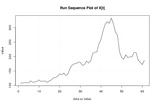
| Dataseries X: | |||||||||||||||||||||||||||||||||||||||||||||||||||||||||||||||||
108,2 108,8 110,2 109,5 109,5 116 111,2 112,1 114 119,1 114,1 115,1 115,4 110,8 116 119,2 126,5 127,8 131,3 140,3 137,3 143 134,5 139,9 159,3 170,4 175 175,8 180,9 180,3 169,6 172,3 184,8 177,7 184,6 211,4 215,3 215,9 244,7 259,3 289 310,9 321 315,1 333,2 314,1 284,7 273,9 216 196,4 190,9 206,4 196,3 199,5 198,9 214,4 214,2 187,6 180,6 172,2 187,2 | |||||||||||||||||||||||||||||||||||||||||||||||||||||||||||||||||
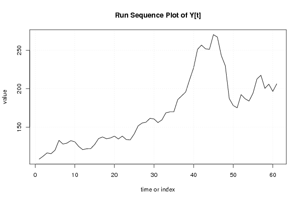
| Dataseries Y: | |||||||||||||||||||||||||||||||||||||||||||||||||||||||||||||||||
108,5 112,3 116,6 115,5 120,1 132,9 128,1 129,3 132,5 131 124,9 120,8 122 122,1 127,4 135,2 137,3 135 136 138,4 134,7 138,4 133,9 133,6 141,2 151,8 155,4 156,6 161,6 160,7 156 159,5 168,7 169,9 169,9 185,9 190,8 195,8 211,9 227,1 251,3 256,7 251,9 251,2 270,3 267,2 243 229,9 187,2 178,2 175,2 192,4 187 184 194,1 212,7 217,5 200,5 205,9 196,5 206,3 | |||||||||||||||||||||||||||||||||||||||||||||||||||||||||||||||||
Tables (Output of Computation) | |||||||||||||||||||||||||||||||||||||||||||||||||||||||||||||||||
| |||||||||||||||||||||||||||||||||||||||||||||||||||||||||||||||||
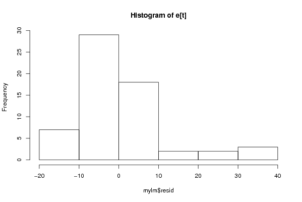
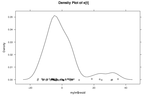
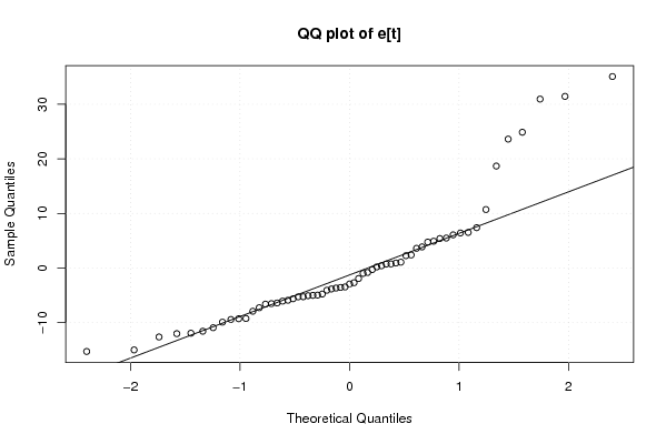
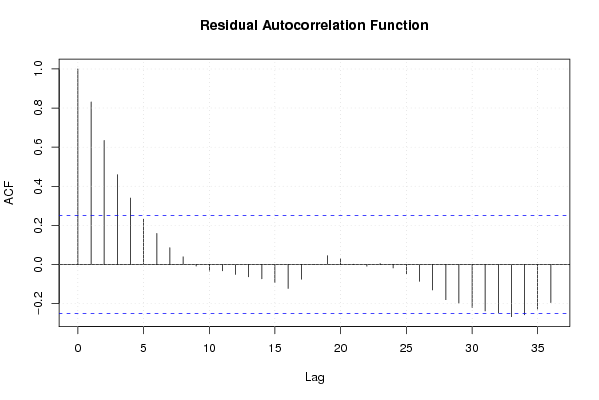
Figures (Output of Computation) | |||||||||||||||||||||||||||||||||||||||||||||||||||||||||||||||||
Input Parameters & R Code | |||||||||||||||||||||||||||||||||||||||||||||||||||||||||||||||||
| Parameters (Session): | |||||||||||||||||||||||||||||||||||||||||||||||||||||||||||||||||
| par1 = 0 ; par2 = 36 ; | |||||||||||||||||||||||||||||||||||||||||||||||||||||||||||||||||
| Parameters (R input): | |||||||||||||||||||||||||||||||||||||||||||||||||||||||||||||||||
| par1 = 0 ; par2 = 36 ; | |||||||||||||||||||||||||||||||||||||||||||||||||||||||||||||||||
| R code (references can be found in the software module): | |||||||||||||||||||||||||||||||||||||||||||||||||||||||||||||||||
par1 <- as.numeric(par1) | |||||||||||||||||||||||||||||||||||||||||||||||||||||||||||||||||