Repository of Reproducible Computations

Free Statistics

of Irreproducible Research!

Author's title

Author

*The author of this computation has been verified*

R Software Module

rwasp_autocorrelation.wasp

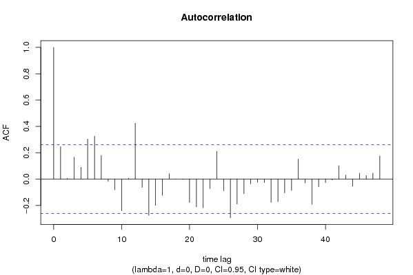
Title produced by software

(Partial) Autocorrelation Function

Date of computation

Fri, 27 Nov 2009 19:00:30 -0700

Cite this page as follows

Statistical Computations at FreeStatistics.org, Office for Research Development and Education, URL https://freestatistics.org/blog/index.php?v=date/2009/Nov/28/t1259373717u897wn2pu3gwgz4.htm/, Retrieved Fri, 03 May 2024 12:14:44 +0000

Statistical Computations at FreeStatistics.org, Office for Research Development and Education, URL https://freestatistics.org/blog/index.php?pk=61361, Retrieved Fri, 03 May 2024 12:14:44 +0000

QR Codes:

Paste this QR Code to cite your computation.

Original text written by user:

IsPrivate?

No (this computation is public)

User-defined keywords

Estimated Impact

174

Family? (F = Feedback message, R = changed R code, M = changed R Module, P = changed Parameters, D = changed Data)

-       [(Partial) Autocorrelation Function] [] [2009-11-28 02:00:30] [dd88bf4749af0c195ad4f54cb428da1c] [Current]
-   P     [(Partial) Autocorrelation Function] [] [2009-11-28 02:11:06] [2f9700e78f159997f527be4a316457f5] 
- RMPD    [Variance Reduction Matrix] [] [2009-11-28 02:18:41] [2f9700e78f159997f527be4a316457f5] 
- RMPD    [Spectral Analysis] [] [2009-11-28 02:35:12] [2f9700e78f159997f527be4a316457f5] 
- RMP     [Spectral Analysis] [] [2009-11-28 02:40:34] [2f9700e78f159997f527be4a316457f5] 
- RMP     [Spectral Analysis] [] [2009-11-28 02:51:41] [2f9700e78f159997f527be4a316457f5] 
- RMPD    [Standard Deviation-Mean Plot] [] [2009-11-28 02:58:50] [2f9700e78f159997f527be4a316457f5] 

Feedback Forum

Post a new message

Dataseries X:

Download CSV

Histogram

Boxplots

Summary of computational transaction
Raw Input	view raw input (R code)
Raw Output	view raw output of R engine
Computing time	2 seconds
R Server	'Gwilym Jenkins' @ 72.249.127.135

\begin{tabular}{lllllllll}
\hline
Summary of computational transaction \tabularnewline
Raw Input & view raw input (R code)  \tabularnewline
Raw Output & view raw output of R engine  \tabularnewline
Computing time & 2 seconds \tabularnewline
R Server & 'Gwilym Jenkins' @ 72.249.127.135 \tabularnewline
\hline
\end{tabular}
%Source: https://freestatistics.org/blog/index.php?pk=61361&T=0

[TABLE]
[ROW][C]Summary of computational transaction[/C][/ROW]
[ROW][C]Raw Input[/C][C]view raw input (R code) [/C][/ROW]
[ROW][C]Raw Output[/C][C]view raw output of R engine [/C][/ROW]
[ROW][C]Computing time[/C][C]2 seconds[/C][/ROW]
[ROW][C]R Server[/C][C]'Gwilym Jenkins' @ 72.249.127.135[/C][/ROW]
[/TABLE]
Source: https://freestatistics.org/blog/index.php?pk=61361&T=0

Globally Unique Identifier (entire table): ba.freestatistics.org/blog/index.php?pk=61361&T=0

As an alternative you can also use a QR Code:

The GUIDs for individual cells are displayed in the table below:

Summary of computational transaction
Raw Input	view raw input (R code)
Raw Output	view raw output of R engine
Computing time	2 seconds
R Server	'Gwilym Jenkins' @ 72.249.127.135

Autocorrelation Function
Time lag k	ACF(k)	T-STAT	P-value
1	0.245923	1.8403	0.035512
2	0.005323	0.0398	0.484184
3	0.166226	1.2439	0.109355
4	0.089428	0.6692	0.253053
5	0.303552	2.2716	0.013487
6	0.325775	2.4379	0.008987
7	0.179394	1.3425	0.092432
8	-0.018427	-0.1379	0.445409
9	-0.080773	-0.6045	0.273993
10	-0.241035	-1.8037	0.038326
11	0.006022	0.0451	0.482109
12	0.423929	3.1724	0.001227
13	-0.063217	-0.4731	0.319
14	-0.275076	-2.0585	0.022104
15	-0.200214	-1.4983	0.06984
16	-0.124195	-0.9294	0.178339
17	0.04128	0.3089	0.379267
18	-0.000539	-0.004	0.498399
19	-0.002837	-0.0212	0.491568
20	-0.177597	-1.329	0.094616
21	-0.210421	-1.5746	0.060486
22	-0.219028	-1.6391	0.053404
23	-0.072588	-0.5432	0.294573
24	0.211109	1.5798	0.059893
25	-0.08836	-0.6612	0.255589
26	-0.293395	-2.1956	0.016141
27	-0.188902	-1.4136	0.081505
28	-0.111733	-0.8361	0.203318
29	-0.036428	-0.2726	0.393081
30	-0.02444	-0.1829	0.42777
31	-0.026889	-0.2012	0.420628
32	-0.17684	-1.3233	0.095549
33	-0.171825	-1.2858	0.101898
34	-0.104841	-0.7846	0.21801
35	-0.086397	-0.6465	0.260288
36	0.151641	1.1348	0.130651
37	-0.029736	-0.2225	0.412359
38	-0.192308	-1.4391	0.077844
39	-0.05771	-0.4319	0.333751
40	-0.026799	-0.2005	0.420892
41	-0.006631	-0.0496	0.480301
42	0.101324	0.7582	0.225743
43	0.030725	0.2299	0.409495
44	-0.05454	-0.4081	0.342363
45	0.044185	0.3306	0.371072
46	0.027095	0.2028	0.420028
47	0.045262	0.3387	0.368047
48	0.176512	1.3209	0.095955

\begin{tabular}{lllllllll}
\hline
Autocorrelation Function \tabularnewline
Time lag k & ACF(k) & T-STAT & P-value \tabularnewline
1 & 0.245923 & 1.8403 & 0.035512 \tabularnewline
2 & 0.005323 & 0.0398 & 0.484184 \tabularnewline
3 & 0.166226 & 1.2439 & 0.109355 \tabularnewline
4 & 0.089428 & 0.6692 & 0.253053 \tabularnewline
5 & 0.303552 & 2.2716 & 0.013487 \tabularnewline
6 & 0.325775 & 2.4379 & 0.008987 \tabularnewline
7 & 0.179394 & 1.3425 & 0.092432 \tabularnewline
8 & -0.018427 & -0.1379 & 0.445409 \tabularnewline
9 & -0.080773 & -0.6045 & 0.273993 \tabularnewline
10 & -0.241035 & -1.8037 & 0.038326 \tabularnewline
11 & 0.006022 & 0.0451 & 0.482109 \tabularnewline
12 & 0.423929 & 3.1724 & 0.001227 \tabularnewline
13 & -0.063217 & -0.4731 & 0.319 \tabularnewline
14 & -0.275076 & -2.0585 & 0.022104 \tabularnewline
15 & -0.200214 & -1.4983 & 0.06984 \tabularnewline
16 & -0.124195 & -0.9294 & 0.178339 \tabularnewline
17 & 0.04128 & 0.3089 & 0.379267 \tabularnewline
18 & -0.000539 & -0.004 & 0.498399 \tabularnewline
19 & -0.002837 & -0.0212 & 0.491568 \tabularnewline
20 & -0.177597 & -1.329 & 0.094616 \tabularnewline
21 & -0.210421 & -1.5746 & 0.060486 \tabularnewline
22 & -0.219028 & -1.6391 & 0.053404 \tabularnewline
23 & -0.072588 & -0.5432 & 0.294573 \tabularnewline
24 & 0.211109 & 1.5798 & 0.059893 \tabularnewline
25 & -0.08836 & -0.6612 & 0.255589 \tabularnewline
26 & -0.293395 & -2.1956 & 0.016141 \tabularnewline
27 & -0.188902 & -1.4136 & 0.081505 \tabularnewline
28 & -0.111733 & -0.8361 & 0.203318 \tabularnewline
29 & -0.036428 & -0.2726 & 0.393081 \tabularnewline
30 & -0.02444 & -0.1829 & 0.42777 \tabularnewline
31 & -0.026889 & -0.2012 & 0.420628 \tabularnewline
32 & -0.17684 & -1.3233 & 0.095549 \tabularnewline
33 & -0.171825 & -1.2858 & 0.101898 \tabularnewline
34 & -0.104841 & -0.7846 & 0.21801 \tabularnewline
35 & -0.086397 & -0.6465 & 0.260288 \tabularnewline
36 & 0.151641 & 1.1348 & 0.130651 \tabularnewline
37 & -0.029736 & -0.2225 & 0.412359 \tabularnewline
38 & -0.192308 & -1.4391 & 0.077844 \tabularnewline
39 & -0.05771 & -0.4319 & 0.333751 \tabularnewline
40 & -0.026799 & -0.2005 & 0.420892 \tabularnewline
41 & -0.006631 & -0.0496 & 0.480301 \tabularnewline
42 & 0.101324 & 0.7582 & 0.225743 \tabularnewline
43 & 0.030725 & 0.2299 & 0.409495 \tabularnewline
44 & -0.05454 & -0.4081 & 0.342363 \tabularnewline
45 & 0.044185 & 0.3306 & 0.371072 \tabularnewline
46 & 0.027095 & 0.2028 & 0.420028 \tabularnewline
47 & 0.045262 & 0.3387 & 0.368047 \tabularnewline
48 & 0.176512 & 1.3209 & 0.095955 \tabularnewline
\hline
\end{tabular}
%Source: https://freestatistics.org/blog/index.php?pk=61361&T=1

[TABLE]
[ROW][C]Autocorrelation Function[/C][/ROW]
[ROW][C]Time lag k[/C][C]ACF(k)[/C][C]T-STAT[/C][C]P-value[/C][/ROW]
[ROW][C]1[/C][C]0.245923[/C][C]1.8403[/C][C]0.035512[/C][/ROW]
[ROW][C]2[/C][C]0.005323[/C][C]0.0398[/C][C]0.484184[/C][/ROW]
[ROW][C]3[/C][C]0.166226[/C][C]1.2439[/C][C]0.109355[/C][/ROW]
[ROW][C]4[/C][C]0.089428[/C][C]0.6692[/C][C]0.253053[/C][/ROW]
[ROW][C]5[/C][C]0.303552[/C][C]2.2716[/C][C]0.013487[/C][/ROW]
[ROW][C]6[/C][C]0.325775[/C][C]2.4379[/C][C]0.008987[/C][/ROW]
[ROW][C]7[/C][C]0.179394[/C][C]1.3425[/C][C]0.092432[/C][/ROW]
[ROW][C]8[/C][C]-0.018427[/C][C]-0.1379[/C][C]0.445409[/C][/ROW]
[ROW][C]9[/C][C]-0.080773[/C][C]-0.6045[/C][C]0.273993[/C][/ROW]
[ROW][C]10[/C][C]-0.241035[/C][C]-1.8037[/C][C]0.038326[/C][/ROW]
[ROW][C]11[/C][C]0.006022[/C][C]0.0451[/C][C]0.482109[/C][/ROW]
[ROW][C]12[/C][C]0.423929[/C][C]3.1724[/C][C]0.001227[/C][/ROW]
[ROW][C]13[/C][C]-0.063217[/C][C]-0.4731[/C][C]0.319[/C][/ROW]
[ROW][C]14[/C][C]-0.275076[/C][C]-2.0585[/C][C]0.022104[/C][/ROW]
[ROW][C]15[/C][C]-0.200214[/C][C]-1.4983[/C][C]0.06984[/C][/ROW]
[ROW][C]16[/C][C]-0.124195[/C][C]-0.9294[/C][C]0.178339[/C][/ROW]
[ROW][C]17[/C][C]0.04128[/C][C]0.3089[/C][C]0.379267[/C][/ROW]
[ROW][C]18[/C][C]-0.000539[/C][C]-0.004[/C][C]0.498399[/C][/ROW]
[ROW][C]19[/C][C]-0.002837[/C][C]-0.0212[/C][C]0.491568[/C][/ROW]
[ROW][C]20[/C][C]-0.177597[/C][C]-1.329[/C][C]0.094616[/C][/ROW]
[ROW][C]21[/C][C]-0.210421[/C][C]-1.5746[/C][C]0.060486[/C][/ROW]
[ROW][C]22[/C][C]-0.219028[/C][C]-1.6391[/C][C]0.053404[/C][/ROW]
[ROW][C]23[/C][C]-0.072588[/C][C]-0.5432[/C][C]0.294573[/C][/ROW]
[ROW][C]24[/C][C]0.211109[/C][C]1.5798[/C][C]0.059893[/C][/ROW]
[ROW][C]25[/C][C]-0.08836[/C][C]-0.6612[/C][C]0.255589[/C][/ROW]
[ROW][C]26[/C][C]-0.293395[/C][C]-2.1956[/C][C]0.016141[/C][/ROW]
[ROW][C]27[/C][C]-0.188902[/C][C]-1.4136[/C][C]0.081505[/C][/ROW]
[ROW][C]28[/C][C]-0.111733[/C][C]-0.8361[/C][C]0.203318[/C][/ROW]
[ROW][C]29[/C][C]-0.036428[/C][C]-0.2726[/C][C]0.393081[/C][/ROW]
[ROW][C]30[/C][C]-0.02444[/C][C]-0.1829[/C][C]0.42777[/C][/ROW]
[ROW][C]31[/C][C]-0.026889[/C][C]-0.2012[/C][C]0.420628[/C][/ROW]
[ROW][C]32[/C][C]-0.17684[/C][C]-1.3233[/C][C]0.095549[/C][/ROW]
[ROW][C]33[/C][C]-0.171825[/C][C]-1.2858[/C][C]0.101898[/C][/ROW]
[ROW][C]34[/C][C]-0.104841[/C][C]-0.7846[/C][C]0.21801[/C][/ROW]
[ROW][C]35[/C][C]-0.086397[/C][C]-0.6465[/C][C]0.260288[/C][/ROW]
[ROW][C]36[/C][C]0.151641[/C][C]1.1348[/C][C]0.130651[/C][/ROW]
[ROW][C]37[/C][C]-0.029736[/C][C]-0.2225[/C][C]0.412359[/C][/ROW]
[ROW][C]38[/C][C]-0.192308[/C][C]-1.4391[/C][C]0.077844[/C][/ROW]
[ROW][C]39[/C][C]-0.05771[/C][C]-0.4319[/C][C]0.333751[/C][/ROW]
[ROW][C]40[/C][C]-0.026799[/C][C]-0.2005[/C][C]0.420892[/C][/ROW]
[ROW][C]41[/C][C]-0.006631[/C][C]-0.0496[/C][C]0.480301[/C][/ROW]
[ROW][C]42[/C][C]0.101324[/C][C]0.7582[/C][C]0.225743[/C][/ROW]
[ROW][C]43[/C][C]0.030725[/C][C]0.2299[/C][C]0.409495[/C][/ROW]
[ROW][C]44[/C][C]-0.05454[/C][C]-0.4081[/C][C]0.342363[/C][/ROW]
[ROW][C]45[/C][C]0.044185[/C][C]0.3306[/C][C]0.371072[/C][/ROW]
[ROW][C]46[/C][C]0.027095[/C][C]0.2028[/C][C]0.420028[/C][/ROW]
[ROW][C]47[/C][C]0.045262[/C][C]0.3387[/C][C]0.368047[/C][/ROW]
[ROW][C]48[/C][C]0.176512[/C][C]1.3209[/C][C]0.095955[/C][/ROW]
[/TABLE]
Source: https://freestatistics.org/blog/index.php?pk=61361&T=1

Globally Unique Identifier (entire table): ba.freestatistics.org/blog/index.php?pk=61361&T=1

As an alternative you can also use a QR Code:

The GUIDs for individual cells are displayed in the table below:

Autocorrelation Function
Time lag k	ACF(k)	T-STAT	P-value
1	0.245923	1.8403	0.035512
2	0.005323	0.0398	0.484184
3	0.166226	1.2439	0.109355
4	0.089428	0.6692	0.253053
5	0.303552	2.2716	0.013487
6	0.325775	2.4379	0.008987
7	0.179394	1.3425	0.092432
8	-0.018427	-0.1379	0.445409
9	-0.080773	-0.6045	0.273993
10	-0.241035	-1.8037	0.038326
11	0.006022	0.0451	0.482109
12	0.423929	3.1724	0.001227
13	-0.063217	-0.4731	0.319
14	-0.275076	-2.0585	0.022104
15	-0.200214	-1.4983	0.06984
16	-0.124195	-0.9294	0.178339
17	0.04128	0.3089	0.379267
18	-0.000539	-0.004	0.498399
19	-0.002837	-0.0212	0.491568
20	-0.177597	-1.329	0.094616
21	-0.210421	-1.5746	0.060486
22	-0.219028	-1.6391	0.053404
23	-0.072588	-0.5432	0.294573
24	0.211109	1.5798	0.059893
25	-0.08836	-0.6612	0.255589
26	-0.293395	-2.1956	0.016141
27	-0.188902	-1.4136	0.081505
28	-0.111733	-0.8361	0.203318
29	-0.036428	-0.2726	0.393081
30	-0.02444	-0.1829	0.42777
31	-0.026889	-0.2012	0.420628
32	-0.17684	-1.3233	0.095549
33	-0.171825	-1.2858	0.101898
34	-0.104841	-0.7846	0.21801
35	-0.086397	-0.6465	0.260288
36	0.151641	1.1348	0.130651
37	-0.029736	-0.2225	0.412359
38	-0.192308	-1.4391	0.077844
39	-0.05771	-0.4319	0.333751
40	-0.026799	-0.2005	0.420892
41	-0.006631	-0.0496	0.480301
42	0.101324	0.7582	0.225743
43	0.030725	0.2299	0.409495
44	-0.05454	-0.4081	0.342363
45	0.044185	0.3306	0.371072
46	0.027095	0.2028	0.420028
47	0.045262	0.3387	0.368047
48	0.176512	1.3209	0.095955

Partial Autocorrelation Function
Time lag k	PACF(k)	T-STAT	P-value
1	0.245923	1.8403	0.035512
2	-0.058705	-0.4393	0.331063
3	0.191477	1.4329	0.078725
4	-0.002472	-0.0185	0.492654
5	0.329171	2.4633	0.008433
6	0.174048	1.3025	0.099046
7	0.135548	1.0144	0.157389
8	-0.164478	-1.2308	0.111764
9	-0.140669	-1.0527	0.148506
10	-0.488401	-3.6549	0.000284
11	-0.072777	-0.5446	0.294092
12	0.405386	3.0336	0.001829
13	-0.026404	-0.1976	0.42204
14	-0.088316	-0.6609	0.255694
15	-0.112913	-0.845	0.200863
16	0.133635	1	0.160798
17	-0.034847	-0.2608	0.397612
18	-0.179683	-1.3446	0.092084
19	0.005029	0.0376	0.485056
20	-0.096109	-0.7192	0.237501
21	0.02835	0.2122	0.416379
22	0.035386	0.2648	0.396066
23	-0.041269	-0.3088	0.379299
24	-0.058505	-0.4378	0.331604
25	-0.05882	-0.4402	0.330754
26	-0.047559	-0.3559	0.361628
27	0.018586	0.1391	0.444942
28	-0.134366	-1.0055	0.15949
29	-0.105534	-0.7897	0.216505
30	-0.003055	-0.0229	0.490921
31	0.039276	0.2939	0.384954
32	-0.011586	-0.0867	0.46561
33	-0.034355	-0.2571	0.399027
34	0.102255	0.7652	0.22368
35	-0.134478	-1.0063	0.159291
36	-0.038051	-0.2847	0.388445
37	-0.047833	-0.3579	0.360865
38	-0.009743	-0.0729	0.471069
39	-0.03507	-0.2624	0.396973
40	-0.037791	-0.2828	0.389185
41	-0.058739	-0.4396	0.330974
42	0.135084	1.0109	0.158212
43	-0.0951	-0.7117	0.239814
44	0.060937	0.456	0.325073
45	0.10309	0.7715	0.221841
46	-0.005539	-0.0414	0.483544
47	-0.006394	-0.0478	0.481003
48	-0.127128	-0.9513	0.172761

\begin{tabular}{lllllllll}
\hline
Partial Autocorrelation Function \tabularnewline
Time lag k & PACF(k) & T-STAT & P-value \tabularnewline
1 & 0.245923 & 1.8403 & 0.035512 \tabularnewline
2 & -0.058705 & -0.4393 & 0.331063 \tabularnewline
3 & 0.191477 & 1.4329 & 0.078725 \tabularnewline
4 & -0.002472 & -0.0185 & 0.492654 \tabularnewline
5 & 0.329171 & 2.4633 & 0.008433 \tabularnewline
6 & 0.174048 & 1.3025 & 0.099046 \tabularnewline
7 & 0.135548 & 1.0144 & 0.157389 \tabularnewline
8 & -0.164478 & -1.2308 & 0.111764 \tabularnewline
9 & -0.140669 & -1.0527 & 0.148506 \tabularnewline
10 & -0.488401 & -3.6549 & 0.000284 \tabularnewline
11 & -0.072777 & -0.5446 & 0.294092 \tabularnewline
12 & 0.405386 & 3.0336 & 0.001829 \tabularnewline
13 & -0.026404 & -0.1976 & 0.42204 \tabularnewline
14 & -0.088316 & -0.6609 & 0.255694 \tabularnewline
15 & -0.112913 & -0.845 & 0.200863 \tabularnewline
16 & 0.133635 & 1 & 0.160798 \tabularnewline
17 & -0.034847 & -0.2608 & 0.397612 \tabularnewline
18 & -0.179683 & -1.3446 & 0.092084 \tabularnewline
19 & 0.005029 & 0.0376 & 0.485056 \tabularnewline
20 & -0.096109 & -0.7192 & 0.237501 \tabularnewline
21 & 0.02835 & 0.2122 & 0.416379 \tabularnewline
22 & 0.035386 & 0.2648 & 0.396066 \tabularnewline
23 & -0.041269 & -0.3088 & 0.379299 \tabularnewline
24 & -0.058505 & -0.4378 & 0.331604 \tabularnewline
25 & -0.05882 & -0.4402 & 0.330754 \tabularnewline
26 & -0.047559 & -0.3559 & 0.361628 \tabularnewline
27 & 0.018586 & 0.1391 & 0.444942 \tabularnewline
28 & -0.134366 & -1.0055 & 0.15949 \tabularnewline
29 & -0.105534 & -0.7897 & 0.216505 \tabularnewline
30 & -0.003055 & -0.0229 & 0.490921 \tabularnewline
31 & 0.039276 & 0.2939 & 0.384954 \tabularnewline
32 & -0.011586 & -0.0867 & 0.46561 \tabularnewline
33 & -0.034355 & -0.2571 & 0.399027 \tabularnewline
34 & 0.102255 & 0.7652 & 0.22368 \tabularnewline
35 & -0.134478 & -1.0063 & 0.159291 \tabularnewline
36 & -0.038051 & -0.2847 & 0.388445 \tabularnewline
37 & -0.047833 & -0.3579 & 0.360865 \tabularnewline
38 & -0.009743 & -0.0729 & 0.471069 \tabularnewline
39 & -0.03507 & -0.2624 & 0.396973 \tabularnewline
40 & -0.037791 & -0.2828 & 0.389185 \tabularnewline
41 & -0.058739 & -0.4396 & 0.330974 \tabularnewline
42 & 0.135084 & 1.0109 & 0.158212 \tabularnewline
43 & -0.0951 & -0.7117 & 0.239814 \tabularnewline
44 & 0.060937 & 0.456 & 0.325073 \tabularnewline
45 & 0.10309 & 0.7715 & 0.221841 \tabularnewline
46 & -0.005539 & -0.0414 & 0.483544 \tabularnewline
47 & -0.006394 & -0.0478 & 0.481003 \tabularnewline
48 & -0.127128 & -0.9513 & 0.172761 \tabularnewline
\hline
\end{tabular}
%Source: https://freestatistics.org/blog/index.php?pk=61361&T=2

[TABLE]
[ROW][C]Partial Autocorrelation Function[/C][/ROW]
[ROW][C]Time lag k[/C][C]PACF(k)[/C][C]T-STAT[/C][C]P-value[/C][/ROW]
[ROW][C]1[/C][C]0.245923[/C][C]1.8403[/C][C]0.035512[/C][/ROW]
[ROW][C]2[/C][C]-0.058705[/C][C]-0.4393[/C][C]0.331063[/C][/ROW]
[ROW][C]3[/C][C]0.191477[/C][C]1.4329[/C][C]0.078725[/C][/ROW]
[ROW][C]4[/C][C]-0.002472[/C][C]-0.0185[/C][C]0.492654[/C][/ROW]
[ROW][C]5[/C][C]0.329171[/C][C]2.4633[/C][C]0.008433[/C][/ROW]
[ROW][C]6[/C][C]0.174048[/C][C]1.3025[/C][C]0.099046[/C][/ROW]
[ROW][C]7[/C][C]0.135548[/C][C]1.0144[/C][C]0.157389[/C][/ROW]
[ROW][C]8[/C][C]-0.164478[/C][C]-1.2308[/C][C]0.111764[/C][/ROW]
[ROW][C]9[/C][C]-0.140669[/C][C]-1.0527[/C][C]0.148506[/C][/ROW]
[ROW][C]10[/C][C]-0.488401[/C][C]-3.6549[/C][C]0.000284[/C][/ROW]
[ROW][C]11[/C][C]-0.072777[/C][C]-0.5446[/C][C]0.294092[/C][/ROW]
[ROW][C]12[/C][C]0.405386[/C][C]3.0336[/C][C]0.001829[/C][/ROW]
[ROW][C]13[/C][C]-0.026404[/C][C]-0.1976[/C][C]0.42204[/C][/ROW]
[ROW][C]14[/C][C]-0.088316[/C][C]-0.6609[/C][C]0.255694[/C][/ROW]
[ROW][C]15[/C][C]-0.112913[/C][C]-0.845[/C][C]0.200863[/C][/ROW]
[ROW][C]16[/C][C]0.133635[/C][C]1[/C][C]0.160798[/C][/ROW]
[ROW][C]17[/C][C]-0.034847[/C][C]-0.2608[/C][C]0.397612[/C][/ROW]
[ROW][C]18[/C][C]-0.179683[/C][C]-1.3446[/C][C]0.092084[/C][/ROW]
[ROW][C]19[/C][C]0.005029[/C][C]0.0376[/C][C]0.485056[/C][/ROW]
[ROW][C]20[/C][C]-0.096109[/C][C]-0.7192[/C][C]0.237501[/C][/ROW]
[ROW][C]21[/C][C]0.02835[/C][C]0.2122[/C][C]0.416379[/C][/ROW]
[ROW][C]22[/C][C]0.035386[/C][C]0.2648[/C][C]0.396066[/C][/ROW]
[ROW][C]23[/C][C]-0.041269[/C][C]-0.3088[/C][C]0.379299[/C][/ROW]
[ROW][C]24[/C][C]-0.058505[/C][C]-0.4378[/C][C]0.331604[/C][/ROW]
[ROW][C]25[/C][C]-0.05882[/C][C]-0.4402[/C][C]0.330754[/C][/ROW]
[ROW][C]26[/C][C]-0.047559[/C][C]-0.3559[/C][C]0.361628[/C][/ROW]
[ROW][C]27[/C][C]0.018586[/C][C]0.1391[/C][C]0.444942[/C][/ROW]
[ROW][C]28[/C][C]-0.134366[/C][C]-1.0055[/C][C]0.15949[/C][/ROW]
[ROW][C]29[/C][C]-0.105534[/C][C]-0.7897[/C][C]0.216505[/C][/ROW]
[ROW][C]30[/C][C]-0.003055[/C][C]-0.0229[/C][C]0.490921[/C][/ROW]
[ROW][C]31[/C][C]0.039276[/C][C]0.2939[/C][C]0.384954[/C][/ROW]
[ROW][C]32[/C][C]-0.011586[/C][C]-0.0867[/C][C]0.46561[/C][/ROW]
[ROW][C]33[/C][C]-0.034355[/C][C]-0.2571[/C][C]0.399027[/C][/ROW]
[ROW][C]34[/C][C]0.102255[/C][C]0.7652[/C][C]0.22368[/C][/ROW]
[ROW][C]35[/C][C]-0.134478[/C][C]-1.0063[/C][C]0.159291[/C][/ROW]
[ROW][C]36[/C][C]-0.038051[/C][C]-0.2847[/C][C]0.388445[/C][/ROW]
[ROW][C]37[/C][C]-0.047833[/C][C]-0.3579[/C][C]0.360865[/C][/ROW]
[ROW][C]38[/C][C]-0.009743[/C][C]-0.0729[/C][C]0.471069[/C][/ROW]
[ROW][C]39[/C][C]-0.03507[/C][C]-0.2624[/C][C]0.396973[/C][/ROW]
[ROW][C]40[/C][C]-0.037791[/C][C]-0.2828[/C][C]0.389185[/C][/ROW]
[ROW][C]41[/C][C]-0.058739[/C][C]-0.4396[/C][C]0.330974[/C][/ROW]
[ROW][C]42[/C][C]0.135084[/C][C]1.0109[/C][C]0.158212[/C][/ROW]
[ROW][C]43[/C][C]-0.0951[/C][C]-0.7117[/C][C]0.239814[/C][/ROW]
[ROW][C]44[/C][C]0.060937[/C][C]0.456[/C][C]0.325073[/C][/ROW]
[ROW][C]45[/C][C]0.10309[/C][C]0.7715[/C][C]0.221841[/C][/ROW]
[ROW][C]46[/C][C]-0.005539[/C][C]-0.0414[/C][C]0.483544[/C][/ROW]
[ROW][C]47[/C][C]-0.006394[/C][C]-0.0478[/C][C]0.481003[/C][/ROW]
[ROW][C]48[/C][C]-0.127128[/C][C]-0.9513[/C][C]0.172761[/C][/ROW]
[/TABLE]
Source: https://freestatistics.org/blog/index.php?pk=61361&T=2

Globally Unique Identifier (entire table): ba.freestatistics.org/blog/index.php?pk=61361&T=2

As an alternative you can also use a QR Code:

The GUIDs for individual cells are displayed in the table below:

Partial Autocorrelation Function
Time lag k	PACF(k)	T-STAT	P-value
1	0.245923	1.8403	0.035512
2	-0.058705	-0.4393	0.331063
3	0.191477	1.4329	0.078725
4	-0.002472	-0.0185	0.492654
5	0.329171	2.4633	0.008433
6	0.174048	1.3025	0.099046
7	0.135548	1.0144	0.157389
8	-0.164478	-1.2308	0.111764
9	-0.140669	-1.0527	0.148506
10	-0.488401	-3.6549	0.000284
11	-0.072777	-0.5446	0.294092
12	0.405386	3.0336	0.001829
13	-0.026404	-0.1976	0.42204
14	-0.088316	-0.6609	0.255694
15	-0.112913	-0.845	0.200863
16	0.133635	1	0.160798
17	-0.034847	-0.2608	0.397612
18	-0.179683	-1.3446	0.092084
19	0.005029	0.0376	0.485056
20	-0.096109	-0.7192	0.237501
21	0.02835	0.2122	0.416379
22	0.035386	0.2648	0.396066
23	-0.041269	-0.3088	0.379299
24	-0.058505	-0.4378	0.331604
25	-0.05882	-0.4402	0.330754
26	-0.047559	-0.3559	0.361628
27	0.018586	0.1391	0.444942
28	-0.134366	-1.0055	0.15949
29	-0.105534	-0.7897	0.216505
30	-0.003055	-0.0229	0.490921
31	0.039276	0.2939	0.384954
32	-0.011586	-0.0867	0.46561
33	-0.034355	-0.2571	0.399027
34	0.102255	0.7652	0.22368
35	-0.134478	-1.0063	0.159291
36	-0.038051	-0.2847	0.388445
37	-0.047833	-0.3579	0.360865
38	-0.009743	-0.0729	0.471069
39	-0.03507	-0.2624	0.396973
40	-0.037791	-0.2828	0.389185
41	-0.058739	-0.4396	0.330974
42	0.135084	1.0109	0.158212
43	-0.0951	-0.7117	0.239814
44	0.060937	0.456	0.325073
45	0.10309	0.7715	0.221841
46	-0.005539	-0.0414	0.483544
47	-0.006394	-0.0478	0.481003
48	-0.127128	-0.9513	0.172761

Figure 1

PNG link

Postscript link

PDF link

Figure 2

PNG link

Postscript link

PDF link

Parameters (Session):

par1 = 48 ; par2 = 1 ; par3 = 0 ; par4 = 0 ; par5 = 12 ; par6 = White Noise ; par7 = 0.95 ;

Parameters (R input):

par1 = 48 ; par2 = 1 ; par3 = 0 ; par4 = 0 ; par5 = 12 ; par6 = White Noise ; par7 = 0.95 ;

R code (references can be found in the software module):

if (par1 == 'Default') {
par1 = 10*log10(length(x))
} else {
par1 <- as.numeric(par1)
}
par2 <- as.numeric(par2)
par3 <- as.numeric(par3)
par4 <- as.numeric(par4)
par5 <- as.numeric(par5)
if (par6 == 'White Noise') par6 <- 'white' else par6 <- 'ma'
par7 <- as.numeric(par7)
if (par2 == 0) {
x <- log(x)
} else {
x <- (x ^ par2 - 1) / par2
}
if (par3 > 0) x <- diff(x,lag=1,difference=par3)
if (par4 > 0) x <- diff(x,lag=par5,difference=par4)
bitmap(file='pic1.png')
racf <- acf(x, par1, main='Autocorrelation', xlab='time lag', ylab='ACF', ci.type=par6, ci=par7, sub=paste('(lambda=',par2,', d=',par3,', D=',par4,', CI=', par7, ', CI type=',par6,')',sep=''))
dev.off()
bitmap(file='pic2.png')
rpacf <- pacf(x,par1,main='Partial Autocorrelation',xlab='lags',ylab='PACF')
dev.off()
(myacf <- c(racf$acf))
(mypacf <- c(rpacf$acf))
lengthx <- length(x)
sqrtn <- sqrt(lengthx)
load(file='createtable')
a<-table.start()
a<-table.row.start(a)
a<-table.element(a,'Autocorrelation Function',4,TRUE)
a<-table.row.end(a)
a<-table.row.start(a)
a<-table.element(a,'Time lag k',header=TRUE)
a<-table.element(a,hyperlink('basics.htm','ACF(k)','click here for more information about the Autocorrelation Function'),header=TRUE)
a<-table.element(a,'T-STAT',header=TRUE)
a<-table.element(a,'P-value',header=TRUE)
a<-table.row.end(a)
for (i in 2:(par1+1)) {
a<-table.row.start(a)
a<-table.element(a,i-1,header=TRUE)
a<-table.element(a,round(myacf[i],6))
mytstat <- myacf[i]*sqrtn
a<-table.element(a,round(mytstat,4))
a<-table.element(a,round(1-pt(abs(mytstat),lengthx),6))
a<-table.row.end(a)
}
a<-table.end(a)
table.save(a,file='mytable.tab')
a<-table.start()
a<-table.row.start(a)
a<-table.element(a,'Partial Autocorrelation Function',4,TRUE)
a<-table.row.end(a)
a<-table.row.start(a)
a<-table.element(a,'Time lag k',header=TRUE)
a<-table.element(a,hyperlink('basics.htm','PACF(k)','click here for more information about the Partial Autocorrelation Function'),header=TRUE)
a<-table.element(a,'T-STAT',header=TRUE)
a<-table.element(a,'P-value',header=TRUE)
a<-table.row.end(a)
for (i in 1:par1) {
a<-table.row.start(a)
a<-table.element(a,i,header=TRUE)
a<-table.element(a,round(mypacf[i],6))
mytstat <- mypacf[i]*sqrtn
a<-table.element(a,round(mytstat,4))
a<-table.element(a,round(1-pt(abs(mytstat),lengthx),6))
a<-table.row.end(a)
}
a<-table.end(a)
table.save(a,file='mytable1.tab')

Free Statistics

Description of Statistical Computation

Tree of Dependent Computations

Dataset

Tables (Output of Computation)

Figures (Output of Computation)

Input Parameters & R Code