Repository of Reproducible Computations

Free Statistics

of Irreproducible Research!

Author's title

Author

*The author of this computation has been verified*

R Software Module

rwasp_autocorrelation.wasp

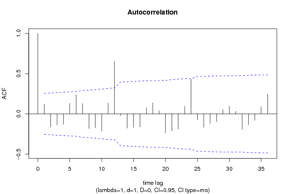
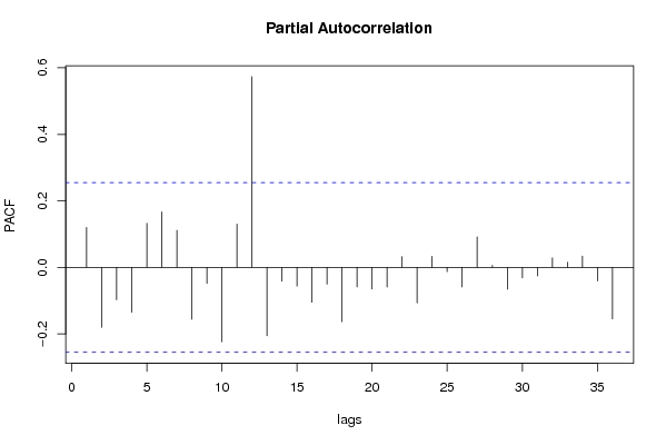
Title produced by software

(Partial) Autocorrelation Function

Date of computation

Fri, 27 Nov 2009 14:32:39 -0700

Cite this page as follows

Statistical Computations at FreeStatistics.org, Office for Research Development and Education, URL https://freestatistics.org/blog/index.php?v=date/2009/Nov/27/t1259357606099aec0pe6v15r3.htm/, Retrieved Mon, 29 Apr 2024 19:54:05 +0000

Statistical Computations at FreeStatistics.org, Office for Research Development and Education, URL https://freestatistics.org/blog/index.php?pk=61291, Retrieved Mon, 29 Apr 2024 19:54:05 +0000

QR Codes:

Paste this QR Code to cite your computation.

Original text written by user:

IsPrivate?

No (this computation is public)

User-defined keywords

Estimated Impact

225

Family? (F = Feedback message, R = changed R code, M = changed R Module, P = changed Parameters, D = changed Data)

-     [Univariate Explorative Data Analysis] [Run Sequence gebo...] [2008-12-12 13:32:37] [76963dc1903f0f612b6153510a3818cf]
- R  D  [Univariate Explorative Data Analysis] [Run Sequence gebo...] [2008-12-17 12:14:40] [76963dc1903f0f612b6153510a3818cf]
-         [Univariate Explorative Data Analysis] [Run Sequence Plot...] [2008-12-22 18:19:51] [1ce0d16c8f4225c977b42c8fa93bc163]
- RMP       [(Partial) Autocorrelation Function] [Identifying Integ...] [2009-11-22 12:16:10] [b98453cac15ba1066b407e146608df68]
-    D        [(Partial) Autocorrelation Function] [] [2009-11-25 17:18:51] [90f6d58d515a4caed6fb4b8be4e11eaa]
-   PD          [(Partial) Autocorrelation Function] [] [2009-11-25 17:25:52] [90f6d58d515a4caed6fb4b8be4e11eaa]
-   P             [(Partial) Autocorrelation Function] [] [2009-11-27 10:21:34] [90f6d58d515a4caed6fb4b8be4e11eaa]
- R  D                [(Partial) Autocorrelation Function] [WorkShop8 (SHW)] [2009-11-27 21:32:39] [2d9a0b3c2f25bb8f387fafb994d0d852] [Current]

Feedback Forum

Post a new message

Dataseries X:

Download CSV

Histogram

Boxplots

Summary of computational transaction
Raw Input	view raw input (R code)
Raw Output	view raw output of R engine
Computing time	1 seconds
R Server	'Gwilym Jenkins' @ 72.249.127.135

\begin{tabular}{lllllllll}
\hline
Summary of computational transaction \tabularnewline
Raw Input & view raw input (R code)  \tabularnewline
Raw Output & view raw output of R engine  \tabularnewline
Computing time & 1 seconds \tabularnewline
R Server & 'Gwilym Jenkins' @ 72.249.127.135 \tabularnewline
\hline
\end{tabular}
%Source: https://freestatistics.org/blog/index.php?pk=61291&T=0

[TABLE]
[ROW][C]Summary of computational transaction[/C][/ROW]
[ROW][C]Raw Input[/C][C]view raw input (R code) [/C][/ROW]
[ROW][C]Raw Output[/C][C]view raw output of R engine [/C][/ROW]
[ROW][C]Computing time[/C][C]1 seconds[/C][/ROW]
[ROW][C]R Server[/C][C]'Gwilym Jenkins' @ 72.249.127.135[/C][/ROW]
[/TABLE]
Source: https://freestatistics.org/blog/index.php?pk=61291&T=0

Globally Unique Identifier (entire table): ba.freestatistics.org/blog/index.php?pk=61291&T=0

As an alternative you can also use a QR Code:

The GUIDs for individual cells are displayed in the table below:

Summary of computational transaction
Raw Input	view raw input (R code)
Raw Output	view raw output of R engine
Computing time	1 seconds
R Server	'Gwilym Jenkins' @ 72.249.127.135

Autocorrelation Function
Time lag k	ACF(k)	T-STAT	P-value
1	0.120322	0.9242	0.179571
2	-0.162827	-1.2507	0.107991
3	-0.137566	-1.0567	0.147486
4	-0.129208	-0.9925	0.162511
5	0.131647	1.0112	0.158024
6	0.240196	1.845	0.035031
7	0.128761	0.989	0.163343
8	-0.183677	-1.4109	0.08177
9	-0.171827	-1.3198	0.095995
10	-0.212559	-1.6327	0.05393
11	0.134164	1.0305	0.153482
12	0.651687	5.0057	3e-06
13	-0.021117	-0.1622	0.43585
14	-0.176951	-1.3592	0.08963
15	-0.169212	-1.2997	0.099372
16	-0.162687	-1.2496	0.108186
17	0.077384	0.5944	0.277259
18	0.137071	1.0529	0.148348
19	0.041921	0.322	0.374296
20	-0.235954	-1.8124	0.037507
21	-0.211179	-1.6221	0.055058
22	-0.189562	-1.4561	0.075339
23	0.09375	0.7201	0.237151
24	0.432419	3.3215	0.00077
25	-0.075555	-0.5804	0.281944
26	-0.16779	-1.2888	0.101246
27	-0.118511	-0.9103	0.183184
28	-0.098393	-0.7558	0.226397
29	0.054869	0.4215	0.337476
30	0.094237	0.7238	0.236011
31	0.031552	0.2424	0.404672
32	-0.193427	-1.4857	0.071336
33	-0.134406	-1.0324	0.153051
34	-0.081395	-0.6252	0.267124
35	0.090715	0.6968	0.244333
36	0.248547	1.9091	0.030557

\begin{tabular}{lllllllll}
\hline
Autocorrelation Function \tabularnewline
Time lag k & ACF(k) & T-STAT & P-value \tabularnewline
1 & 0.120322 & 0.9242 & 0.179571 \tabularnewline
2 & -0.162827 & -1.2507 & 0.107991 \tabularnewline
3 & -0.137566 & -1.0567 & 0.147486 \tabularnewline
4 & -0.129208 & -0.9925 & 0.162511 \tabularnewline
5 & 0.131647 & 1.0112 & 0.158024 \tabularnewline
6 & 0.240196 & 1.845 & 0.035031 \tabularnewline
7 & 0.128761 & 0.989 & 0.163343 \tabularnewline
8 & -0.183677 & -1.4109 & 0.08177 \tabularnewline
9 & -0.171827 & -1.3198 & 0.095995 \tabularnewline
10 & -0.212559 & -1.6327 & 0.05393 \tabularnewline
11 & 0.134164 & 1.0305 & 0.153482 \tabularnewline
12 & 0.651687 & 5.0057 & 3e-06 \tabularnewline
13 & -0.021117 & -0.1622 & 0.43585 \tabularnewline
14 & -0.176951 & -1.3592 & 0.08963 \tabularnewline
15 & -0.169212 & -1.2997 & 0.099372 \tabularnewline
16 & -0.162687 & -1.2496 & 0.108186 \tabularnewline
17 & 0.077384 & 0.5944 & 0.277259 \tabularnewline
18 & 0.137071 & 1.0529 & 0.148348 \tabularnewline
19 & 0.041921 & 0.322 & 0.374296 \tabularnewline
20 & -0.235954 & -1.8124 & 0.037507 \tabularnewline
21 & -0.211179 & -1.6221 & 0.055058 \tabularnewline
22 & -0.189562 & -1.4561 & 0.075339 \tabularnewline
23 & 0.09375 & 0.7201 & 0.237151 \tabularnewline
24 & 0.432419 & 3.3215 & 0.00077 \tabularnewline
25 & -0.075555 & -0.5804 & 0.281944 \tabularnewline
26 & -0.16779 & -1.2888 & 0.101246 \tabularnewline
27 & -0.118511 & -0.9103 & 0.183184 \tabularnewline
28 & -0.098393 & -0.7558 & 0.226397 \tabularnewline
29 & 0.054869 & 0.4215 & 0.337476 \tabularnewline
30 & 0.094237 & 0.7238 & 0.236011 \tabularnewline
31 & 0.031552 & 0.2424 & 0.404672 \tabularnewline
32 & -0.193427 & -1.4857 & 0.071336 \tabularnewline
33 & -0.134406 & -1.0324 & 0.153051 \tabularnewline
34 & -0.081395 & -0.6252 & 0.267124 \tabularnewline
35 & 0.090715 & 0.6968 & 0.244333 \tabularnewline
36 & 0.248547 & 1.9091 & 0.030557 \tabularnewline
\hline
\end{tabular}
%Source: https://freestatistics.org/blog/index.php?pk=61291&T=1

[TABLE]
[ROW][C]Autocorrelation Function[/C][/ROW]
[ROW][C]Time lag k[/C][C]ACF(k)[/C][C]T-STAT[/C][C]P-value[/C][/ROW]
[ROW][C]1[/C][C]0.120322[/C][C]0.9242[/C][C]0.179571[/C][/ROW]
[ROW][C]2[/C][C]-0.162827[/C][C]-1.2507[/C][C]0.107991[/C][/ROW]
[ROW][C]3[/C][C]-0.137566[/C][C]-1.0567[/C][C]0.147486[/C][/ROW]
[ROW][C]4[/C][C]-0.129208[/C][C]-0.9925[/C][C]0.162511[/C][/ROW]
[ROW][C]5[/C][C]0.131647[/C][C]1.0112[/C][C]0.158024[/C][/ROW]
[ROW][C]6[/C][C]0.240196[/C][C]1.845[/C][C]0.035031[/C][/ROW]
[ROW][C]7[/C][C]0.128761[/C][C]0.989[/C][C]0.163343[/C][/ROW]
[ROW][C]8[/C][C]-0.183677[/C][C]-1.4109[/C][C]0.08177[/C][/ROW]
[ROW][C]9[/C][C]-0.171827[/C][C]-1.3198[/C][C]0.095995[/C][/ROW]
[ROW][C]10[/C][C]-0.212559[/C][C]-1.6327[/C][C]0.05393[/C][/ROW]
[ROW][C]11[/C][C]0.134164[/C][C]1.0305[/C][C]0.153482[/C][/ROW]
[ROW][C]12[/C][C]0.651687[/C][C]5.0057[/C][C]3e-06[/C][/ROW]
[ROW][C]13[/C][C]-0.021117[/C][C]-0.1622[/C][C]0.43585[/C][/ROW]
[ROW][C]14[/C][C]-0.176951[/C][C]-1.3592[/C][C]0.08963[/C][/ROW]
[ROW][C]15[/C][C]-0.169212[/C][C]-1.2997[/C][C]0.099372[/C][/ROW]
[ROW][C]16[/C][C]-0.162687[/C][C]-1.2496[/C][C]0.108186[/C][/ROW]
[ROW][C]17[/C][C]0.077384[/C][C]0.5944[/C][C]0.277259[/C][/ROW]
[ROW][C]18[/C][C]0.137071[/C][C]1.0529[/C][C]0.148348[/C][/ROW]
[ROW][C]19[/C][C]0.041921[/C][C]0.322[/C][C]0.374296[/C][/ROW]
[ROW][C]20[/C][C]-0.235954[/C][C]-1.8124[/C][C]0.037507[/C][/ROW]
[ROW][C]21[/C][C]-0.211179[/C][C]-1.6221[/C][C]0.055058[/C][/ROW]
[ROW][C]22[/C][C]-0.189562[/C][C]-1.4561[/C][C]0.075339[/C][/ROW]
[ROW][C]23[/C][C]0.09375[/C][C]0.7201[/C][C]0.237151[/C][/ROW]
[ROW][C]24[/C][C]0.432419[/C][C]3.3215[/C][C]0.00077[/C][/ROW]
[ROW][C]25[/C][C]-0.075555[/C][C]-0.5804[/C][C]0.281944[/C][/ROW]
[ROW][C]26[/C][C]-0.16779[/C][C]-1.2888[/C][C]0.101246[/C][/ROW]
[ROW][C]27[/C][C]-0.118511[/C][C]-0.9103[/C][C]0.183184[/C][/ROW]
[ROW][C]28[/C][C]-0.098393[/C][C]-0.7558[/C][C]0.226397[/C][/ROW]
[ROW][C]29[/C][C]0.054869[/C][C]0.4215[/C][C]0.337476[/C][/ROW]
[ROW][C]30[/C][C]0.094237[/C][C]0.7238[/C][C]0.236011[/C][/ROW]
[ROW][C]31[/C][C]0.031552[/C][C]0.2424[/C][C]0.404672[/C][/ROW]
[ROW][C]32[/C][C]-0.193427[/C][C]-1.4857[/C][C]0.071336[/C][/ROW]
[ROW][C]33[/C][C]-0.134406[/C][C]-1.0324[/C][C]0.153051[/C][/ROW]
[ROW][C]34[/C][C]-0.081395[/C][C]-0.6252[/C][C]0.267124[/C][/ROW]
[ROW][C]35[/C][C]0.090715[/C][C]0.6968[/C][C]0.244333[/C][/ROW]
[ROW][C]36[/C][C]0.248547[/C][C]1.9091[/C][C]0.030557[/C][/ROW]
[/TABLE]
Source: https://freestatistics.org/blog/index.php?pk=61291&T=1

Globally Unique Identifier (entire table): ba.freestatistics.org/blog/index.php?pk=61291&T=1

As an alternative you can also use a QR Code:

The GUIDs for individual cells are displayed in the table below:

Autocorrelation Function
Time lag k	ACF(k)	T-STAT	P-value
1	0.120322	0.9242	0.179571
2	-0.162827	-1.2507	0.107991
3	-0.137566	-1.0567	0.147486
4	-0.129208	-0.9925	0.162511
5	0.131647	1.0112	0.158024
6	0.240196	1.845	0.035031
7	0.128761	0.989	0.163343
8	-0.183677	-1.4109	0.08177
9	-0.171827	-1.3198	0.095995
10	-0.212559	-1.6327	0.05393
11	0.134164	1.0305	0.153482
12	0.651687	5.0057	3e-06
13	-0.021117	-0.1622	0.43585
14	-0.176951	-1.3592	0.08963
15	-0.169212	-1.2997	0.099372
16	-0.162687	-1.2496	0.108186
17	0.077384	0.5944	0.277259
18	0.137071	1.0529	0.148348
19	0.041921	0.322	0.374296
20	-0.235954	-1.8124	0.037507
21	-0.211179	-1.6221	0.055058
22	-0.189562	-1.4561	0.075339
23	0.09375	0.7201	0.237151
24	0.432419	3.3215	0.00077
25	-0.075555	-0.5804	0.281944
26	-0.16779	-1.2888	0.101246
27	-0.118511	-0.9103	0.183184
28	-0.098393	-0.7558	0.226397
29	0.054869	0.4215	0.337476
30	0.094237	0.7238	0.236011
31	0.031552	0.2424	0.404672
32	-0.193427	-1.4857	0.071336
33	-0.134406	-1.0324	0.153051
34	-0.081395	-0.6252	0.267124
35	0.090715	0.6968	0.244333
36	0.248547	1.9091	0.030557

Partial Autocorrelation Function
Time lag k	PACF(k)	T-STAT	P-value
1	0.120322	0.9242	0.179571
2	-0.179909	-1.3819	0.086105
3	-0.097316	-0.7475	0.228866
4	-0.134896	-1.0362	0.152179
5	0.132866	1.0206	0.155814
6	0.167078	1.2834	0.102193
7	0.111449	0.8561	0.197716
8	-0.155955	-1.1979	0.11787
9	-0.047821	-0.3673	0.357346
10	-0.223623	-1.7177	0.04555
11	0.130353	1.0013	0.160395
12	0.573355	4.404	2.3e-05
13	-0.205631	-1.5795	0.059786
14	-0.041699	-0.3203	0.374937
15	-0.056477	-0.4338	0.333005
16	-0.104582	-0.8033	0.21251
17	-0.050512	-0.388	0.349711
18	-0.163405	-1.2551	0.107188
19	-0.058987	-0.4531	0.326073
20	-0.065009	-0.4993	0.309697
21	-0.059381	-0.4561	0.324991
22	0.032456	0.2493	0.401996
23	-0.106834	-0.8206	0.207587
24	0.033158	0.2547	0.399923
25	-0.012966	-0.0996	0.460503
26	-0.058681	-0.4507	0.326915
27	0.091621	0.7038	0.242177
28	0.005895	0.0453	0.482018
29	-0.065519	-0.5033	0.308328
30	-0.031791	-0.2442	0.403965
31	-0.02589	-0.1989	0.421525
32	0.028782	0.2211	0.412897
33	0.015534	0.1193	0.452713
34	0.033976	0.261	0.39751
35	-0.040924	-0.3143	0.377186
36	-0.154918	-1.19	0.119416

\begin{tabular}{lllllllll}
\hline
Partial Autocorrelation Function \tabularnewline
Time lag k & PACF(k) & T-STAT & P-value \tabularnewline
1 & 0.120322 & 0.9242 & 0.179571 \tabularnewline
2 & -0.179909 & -1.3819 & 0.086105 \tabularnewline
3 & -0.097316 & -0.7475 & 0.228866 \tabularnewline
4 & -0.134896 & -1.0362 & 0.152179 \tabularnewline
5 & 0.132866 & 1.0206 & 0.155814 \tabularnewline
6 & 0.167078 & 1.2834 & 0.102193 \tabularnewline
7 & 0.111449 & 0.8561 & 0.197716 \tabularnewline
8 & -0.155955 & -1.1979 & 0.11787 \tabularnewline
9 & -0.047821 & -0.3673 & 0.357346 \tabularnewline
10 & -0.223623 & -1.7177 & 0.04555 \tabularnewline
11 & 0.130353 & 1.0013 & 0.160395 \tabularnewline
12 & 0.573355 & 4.404 & 2.3e-05 \tabularnewline
13 & -0.205631 & -1.5795 & 0.059786 \tabularnewline
14 & -0.041699 & -0.3203 & 0.374937 \tabularnewline
15 & -0.056477 & -0.4338 & 0.333005 \tabularnewline
16 & -0.104582 & -0.8033 & 0.21251 \tabularnewline
17 & -0.050512 & -0.388 & 0.349711 \tabularnewline
18 & -0.163405 & -1.2551 & 0.107188 \tabularnewline
19 & -0.058987 & -0.4531 & 0.326073 \tabularnewline
20 & -0.065009 & -0.4993 & 0.309697 \tabularnewline
21 & -0.059381 & -0.4561 & 0.324991 \tabularnewline
22 & 0.032456 & 0.2493 & 0.401996 \tabularnewline
23 & -0.106834 & -0.8206 & 0.207587 \tabularnewline
24 & 0.033158 & 0.2547 & 0.399923 \tabularnewline
25 & -0.012966 & -0.0996 & 0.460503 \tabularnewline
26 & -0.058681 & -0.4507 & 0.326915 \tabularnewline
27 & 0.091621 & 0.7038 & 0.242177 \tabularnewline
28 & 0.005895 & 0.0453 & 0.482018 \tabularnewline
29 & -0.065519 & -0.5033 & 0.308328 \tabularnewline
30 & -0.031791 & -0.2442 & 0.403965 \tabularnewline
31 & -0.02589 & -0.1989 & 0.421525 \tabularnewline
32 & 0.028782 & 0.2211 & 0.412897 \tabularnewline
33 & 0.015534 & 0.1193 & 0.452713 \tabularnewline
34 & 0.033976 & 0.261 & 0.39751 \tabularnewline
35 & -0.040924 & -0.3143 & 0.377186 \tabularnewline
36 & -0.154918 & -1.19 & 0.119416 \tabularnewline
\hline
\end{tabular}
%Source: https://freestatistics.org/blog/index.php?pk=61291&T=2

[TABLE]
[ROW][C]Partial Autocorrelation Function[/C][/ROW]
[ROW][C]Time lag k[/C][C]PACF(k)[/C][C]T-STAT[/C][C]P-value[/C][/ROW]
[ROW][C]1[/C][C]0.120322[/C][C]0.9242[/C][C]0.179571[/C][/ROW]
[ROW][C]2[/C][C]-0.179909[/C][C]-1.3819[/C][C]0.086105[/C][/ROW]
[ROW][C]3[/C][C]-0.097316[/C][C]-0.7475[/C][C]0.228866[/C][/ROW]
[ROW][C]4[/C][C]-0.134896[/C][C]-1.0362[/C][C]0.152179[/C][/ROW]
[ROW][C]5[/C][C]0.132866[/C][C]1.0206[/C][C]0.155814[/C][/ROW]
[ROW][C]6[/C][C]0.167078[/C][C]1.2834[/C][C]0.102193[/C][/ROW]
[ROW][C]7[/C][C]0.111449[/C][C]0.8561[/C][C]0.197716[/C][/ROW]
[ROW][C]8[/C][C]-0.155955[/C][C]-1.1979[/C][C]0.11787[/C][/ROW]
[ROW][C]9[/C][C]-0.047821[/C][C]-0.3673[/C][C]0.357346[/C][/ROW]
[ROW][C]10[/C][C]-0.223623[/C][C]-1.7177[/C][C]0.04555[/C][/ROW]
[ROW][C]11[/C][C]0.130353[/C][C]1.0013[/C][C]0.160395[/C][/ROW]
[ROW][C]12[/C][C]0.573355[/C][C]4.404[/C][C]2.3e-05[/C][/ROW]
[ROW][C]13[/C][C]-0.205631[/C][C]-1.5795[/C][C]0.059786[/C][/ROW]
[ROW][C]14[/C][C]-0.041699[/C][C]-0.3203[/C][C]0.374937[/C][/ROW]
[ROW][C]15[/C][C]-0.056477[/C][C]-0.4338[/C][C]0.333005[/C][/ROW]
[ROW][C]16[/C][C]-0.104582[/C][C]-0.8033[/C][C]0.21251[/C][/ROW]
[ROW][C]17[/C][C]-0.050512[/C][C]-0.388[/C][C]0.349711[/C][/ROW]
[ROW][C]18[/C][C]-0.163405[/C][C]-1.2551[/C][C]0.107188[/C][/ROW]
[ROW][C]19[/C][C]-0.058987[/C][C]-0.4531[/C][C]0.326073[/C][/ROW]
[ROW][C]20[/C][C]-0.065009[/C][C]-0.4993[/C][C]0.309697[/C][/ROW]
[ROW][C]21[/C][C]-0.059381[/C][C]-0.4561[/C][C]0.324991[/C][/ROW]
[ROW][C]22[/C][C]0.032456[/C][C]0.2493[/C][C]0.401996[/C][/ROW]
[ROW][C]23[/C][C]-0.106834[/C][C]-0.8206[/C][C]0.207587[/C][/ROW]
[ROW][C]24[/C][C]0.033158[/C][C]0.2547[/C][C]0.399923[/C][/ROW]
[ROW][C]25[/C][C]-0.012966[/C][C]-0.0996[/C][C]0.460503[/C][/ROW]
[ROW][C]26[/C][C]-0.058681[/C][C]-0.4507[/C][C]0.326915[/C][/ROW]
[ROW][C]27[/C][C]0.091621[/C][C]0.7038[/C][C]0.242177[/C][/ROW]
[ROW][C]28[/C][C]0.005895[/C][C]0.0453[/C][C]0.482018[/C][/ROW]
[ROW][C]29[/C][C]-0.065519[/C][C]-0.5033[/C][C]0.308328[/C][/ROW]
[ROW][C]30[/C][C]-0.031791[/C][C]-0.2442[/C][C]0.403965[/C][/ROW]
[ROW][C]31[/C][C]-0.02589[/C][C]-0.1989[/C][C]0.421525[/C][/ROW]
[ROW][C]32[/C][C]0.028782[/C][C]0.2211[/C][C]0.412897[/C][/ROW]
[ROW][C]33[/C][C]0.015534[/C][C]0.1193[/C][C]0.452713[/C][/ROW]
[ROW][C]34[/C][C]0.033976[/C][C]0.261[/C][C]0.39751[/C][/ROW]
[ROW][C]35[/C][C]-0.040924[/C][C]-0.3143[/C][C]0.377186[/C][/ROW]
[ROW][C]36[/C][C]-0.154918[/C][C]-1.19[/C][C]0.119416[/C][/ROW]
[/TABLE]
Source: https://freestatistics.org/blog/index.php?pk=61291&T=2

Globally Unique Identifier (entire table): ba.freestatistics.org/blog/index.php?pk=61291&T=2

As an alternative you can also use a QR Code:

The GUIDs for individual cells are displayed in the table below:

Partial Autocorrelation Function
Time lag k	PACF(k)	T-STAT	P-value
1	0.120322	0.9242	0.179571
2	-0.179909	-1.3819	0.086105
3	-0.097316	-0.7475	0.228866
4	-0.134896	-1.0362	0.152179
5	0.132866	1.0206	0.155814
6	0.167078	1.2834	0.102193
7	0.111449	0.8561	0.197716
8	-0.155955	-1.1979	0.11787
9	-0.047821	-0.3673	0.357346
10	-0.223623	-1.7177	0.04555
11	0.130353	1.0013	0.160395
12	0.573355	4.404	2.3e-05
13	-0.205631	-1.5795	0.059786
14	-0.041699	-0.3203	0.374937
15	-0.056477	-0.4338	0.333005
16	-0.104582	-0.8033	0.21251
17	-0.050512	-0.388	0.349711
18	-0.163405	-1.2551	0.107188
19	-0.058987	-0.4531	0.326073
20	-0.065009	-0.4993	0.309697
21	-0.059381	-0.4561	0.324991
22	0.032456	0.2493	0.401996
23	-0.106834	-0.8206	0.207587
24	0.033158	0.2547	0.399923
25	-0.012966	-0.0996	0.460503
26	-0.058681	-0.4507	0.326915
27	0.091621	0.7038	0.242177
28	0.005895	0.0453	0.482018
29	-0.065519	-0.5033	0.308328
30	-0.031791	-0.2442	0.403965
31	-0.02589	-0.1989	0.421525
32	0.028782	0.2211	0.412897
33	0.015534	0.1193	0.452713
34	0.033976	0.261	0.39751
35	-0.040924	-0.3143	0.377186
36	-0.154918	-1.19	0.119416

Figure 1

PNG link

Postscript link

PDF link

Figure 2

PNG link

Postscript link

PDF link

Parameters (Session):

par1 = 36 ; par2 = 1 ; par3 = 1 ; par4 = 0 ; par5 = 12 ; par6 = MA ; par7 = 0.95 ;

Parameters (R input):

par1 = 36 ; par2 = 1 ; par3 = 1 ; par4 = 0 ; par5 = 12 ; par6 = MA ; par7 = 0.95 ;

R code (references can be found in the software module):

if (par1 == 'Default') {
par1 = 10*log10(length(x))
} else {
par1 <- as.numeric(par1)
}
par2 <- as.numeric(par2)
par3 <- as.numeric(par3)
par4 <- as.numeric(par4)
par5 <- as.numeric(par5)
if (par6 == 'White Noise') par6 <- 'white' else par6 <- 'ma'
par7 <- as.numeric(par7)
if (par2 == 0) {
x <- log(x)
} else {
x <- (x ^ par2 - 1) / par2
}
if (par3 > 0) x <- diff(x,lag=1,difference=par3)
if (par4 > 0) x <- diff(x,lag=par5,difference=par4)
bitmap(file='pic1.png')
racf <- acf(x, par1, main='Autocorrelation', xlab='time lag', ylab='ACF', ci.type=par6, ci=par7, sub=paste('(lambda=',par2,', d=',par3,', D=',par4,', CI=', par7, ', CI type=',par6,')',sep=''))
dev.off()
bitmap(file='pic2.png')
rpacf <- pacf(x,par1,main='Partial Autocorrelation',xlab='lags',ylab='PACF')
dev.off()
(myacf <- c(racf$acf))
(mypacf <- c(rpacf$acf))
lengthx <- length(x)
sqrtn <- sqrt(lengthx)
load(file='createtable')
a<-table.start()
a<-table.row.start(a)
a<-table.element(a,'Autocorrelation Function',4,TRUE)
a<-table.row.end(a)
a<-table.row.start(a)
a<-table.element(a,'Time lag k',header=TRUE)
a<-table.element(a,hyperlink('basics.htm','ACF(k)','click here for more information about the Autocorrelation Function'),header=TRUE)
a<-table.element(a,'T-STAT',header=TRUE)
a<-table.element(a,'P-value',header=TRUE)
a<-table.row.end(a)
for (i in 2:(par1+1)) {
a<-table.row.start(a)
a<-table.element(a,i-1,header=TRUE)
a<-table.element(a,round(myacf[i],6))
mytstat <- myacf[i]*sqrtn
a<-table.element(a,round(mytstat,4))
a<-table.element(a,round(1-pt(abs(mytstat),lengthx),6))
a<-table.row.end(a)
}
a<-table.end(a)
table.save(a,file='mytable.tab')
a<-table.start()
a<-table.row.start(a)
a<-table.element(a,'Partial Autocorrelation Function',4,TRUE)
a<-table.row.end(a)
a<-table.row.start(a)
a<-table.element(a,'Time lag k',header=TRUE)
a<-table.element(a,hyperlink('basics.htm','PACF(k)','click here for more information about the Partial Autocorrelation Function'),header=TRUE)
a<-table.element(a,'T-STAT',header=TRUE)
a<-table.element(a,'P-value',header=TRUE)
a<-table.row.end(a)
for (i in 1:par1) {
a<-table.row.start(a)
a<-table.element(a,i,header=TRUE)
a<-table.element(a,round(mypacf[i],6))
mytstat <- mypacf[i]*sqrtn
a<-table.element(a,round(mytstat,4))
a<-table.element(a,round(1-pt(abs(mytstat),lengthx),6))
a<-table.row.end(a)
}
a<-table.end(a)
table.save(a,file='mytable1.tab')

Free Statistics

Description of Statistical Computation

Tree of Dependent Computations

Dataset

Tables (Output of Computation)

Figures (Output of Computation)

Input Parameters & R Code