Repository of Reproducible Computations

Free Statistics

of Irreproducible Research!

Author's title

Author

*The author of this computation has been verified*

R Software Module

rwasp_autocorrelation.wasp

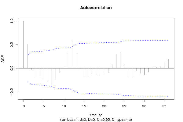
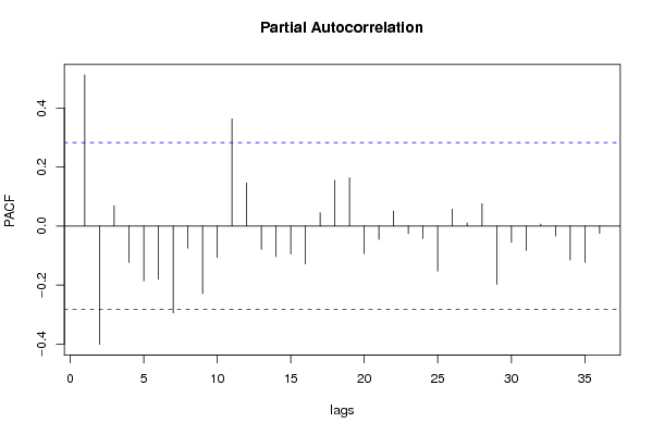
Title produced by software

(Partial) Autocorrelation Function

Date of computation

Fri, 27 Nov 2009 07:23:53 -0700

Cite this page as follows

Statistical Computations at FreeStatistics.org, Office for Research Development and Education, URL https://freestatistics.org/blog/index.php?v=date/2009/Nov/27/t125933195642qfgftiryysvoo.htm/, Retrieved Mon, 29 Apr 2024 18:01:40 +0000

Statistical Computations at FreeStatistics.org, Office for Research Development and Education, URL https://freestatistics.org/blog/index.php?pk=60811, Retrieved Mon, 29 Apr 2024 18:01:40 +0000

QR Codes:

Paste this QR Code to cite your computation.

Original text written by user:

IsPrivate?

No (this computation is public)

User-defined keywords

Estimated Impact

125

Family? (F = Feedback message, R = changed R code, M = changed R Module, P = changed Parameters, D = changed Data)

-     [Univariate Explorative Data Analysis] [Run Sequence gebo...] [2008-12-12 13:32:37] [76963dc1903f0f612b6153510a3818cf]
- R  D  [Univariate Explorative Data Analysis] [Run Sequence gebo...] [2008-12-17 12:14:40] [76963dc1903f0f612b6153510a3818cf]
-         [Univariate Explorative Data Analysis] [Run Sequence Plot...] [2008-12-22 18:19:51] [1ce0d16c8f4225c977b42c8fa93bc163]
- RMP       [(Partial) Autocorrelation Function] [Identifying Integ...] [2009-11-22 12:16:10] [b98453cac15ba1066b407e146608df68]
- R  D          [(Partial) Autocorrelation Function] [] [2009-11-27 14:23:53] [21edaefb91319406e70b6c03c71b58b3] [Current]
-   P             [(Partial) Autocorrelation Function] [] [2009-11-27 14:28:24] [ea26ab7ea3bba830cfeb08d06278d52c] 
-   P               [(Partial) Autocorrelation Function] [] [2009-11-27 14:34:22] [ea26ab7ea3bba830cfeb08d06278d52c] 

Feedback Forum

Post a new message

Dataseries X:

Download CSV

Histogram

Boxplots

Summary of computational transaction
Raw Input	view raw input (R code)
Raw Output	view raw output of R engine
Computing time	1 seconds
R Server	'Gwilym Jenkins' @ 72.249.127.135

\begin{tabular}{lllllllll}
\hline
Summary of computational transaction \tabularnewline
Raw Input & view raw input (R code)  \tabularnewline
Raw Output & view raw output of R engine  \tabularnewline
Computing time & 1 seconds \tabularnewline
R Server & 'Gwilym Jenkins' @ 72.249.127.135 \tabularnewline
\hline
\end{tabular}
%Source: https://freestatistics.org/blog/index.php?pk=60811&T=0

[TABLE]
[ROW][C]Summary of computational transaction[/C][/ROW]
[ROW][C]Raw Input[/C][C]view raw input (R code) [/C][/ROW]
[ROW][C]Raw Output[/C][C]view raw output of R engine [/C][/ROW]
[ROW][C]Computing time[/C][C]1 seconds[/C][/ROW]
[ROW][C]R Server[/C][C]'Gwilym Jenkins' @ 72.249.127.135[/C][/ROW]
[/TABLE]
Source: https://freestatistics.org/blog/index.php?pk=60811&T=0

Globally Unique Identifier (entire table): ba.freestatistics.org/blog/index.php?pk=60811&T=0

As an alternative you can also use a QR Code:

The GUIDs for individual cells are displayed in the table below:

Summary of computational transaction
Raw Input	view raw input (R code)
Raw Output	view raw output of R engine
Computing time	1 seconds
R Server	'Gwilym Jenkins' @ 72.249.127.135

Autocorrelation Function
Time lag k	ACF(k)	T-STAT	P-value
1	0.511898	3.5465	0.000442
2	-0.034153	-0.2366	0.40698
3	-0.187524	-1.2992	0.10004
4	-0.165277	-1.1451	0.128929
5	-0.211433	-1.4648	0.074741
6	-0.289715	-2.0072	0.025188
7	-0.359206	-2.4887	0.008172
8	-0.248261	-1.72	0.045937
9	-0.095888	-0.6643	0.254828
10	0.027702	0.1919	0.424305
11	0.350223	2.4264	0.009527
12	0.571657	3.9606	0.000123
13	0.347567	2.408	0.009965
14	-0.028899	-0.2002	0.421078
15	-0.186111	-1.2894	0.101716
16	-0.189195	-1.3108	0.098085
17	-0.123253	-0.8539	0.198696
18	-0.106936	-0.7409	0.23119
19	-0.131443	-0.9107	0.183512
20	-0.151288	-1.0482	0.149909
21	-0.094038	-0.6515	0.258911
22	0.079885	0.5535	0.29126
23	0.306374	2.1226	0.019485
24	0.341483	2.3659	0.011037
25	0.058902	0.4081	0.342513
26	-0.16883	-1.1697	0.123951
27	-0.170778	-1.1832	0.121282
28	-0.058385	-0.4045	0.343821
29	-0.105494	-0.7309	0.234202
30	-0.134334	-0.9307	0.178334
31	-0.082061	-0.5685	0.286161
32	0.009712	0.0673	0.473316
33	0.022746	0.1576	0.43772
34	0.037367	0.2589	0.398415
35	0.118742	0.8227	0.207381
36	0.189008	1.3095	0.098302

\begin{tabular}{lllllllll}
\hline
Autocorrelation Function \tabularnewline
Time lag k & ACF(k) & T-STAT & P-value \tabularnewline
1 & 0.511898 & 3.5465 & 0.000442 \tabularnewline
2 & -0.034153 & -0.2366 & 0.40698 \tabularnewline
3 & -0.187524 & -1.2992 & 0.10004 \tabularnewline
4 & -0.165277 & -1.1451 & 0.128929 \tabularnewline
5 & -0.211433 & -1.4648 & 0.074741 \tabularnewline
6 & -0.289715 & -2.0072 & 0.025188 \tabularnewline
7 & -0.359206 & -2.4887 & 0.008172 \tabularnewline
8 & -0.248261 & -1.72 & 0.045937 \tabularnewline
9 & -0.095888 & -0.6643 & 0.254828 \tabularnewline
10 & 0.027702 & 0.1919 & 0.424305 \tabularnewline
11 & 0.350223 & 2.4264 & 0.009527 \tabularnewline
12 & 0.571657 & 3.9606 & 0.000123 \tabularnewline
13 & 0.347567 & 2.408 & 0.009965 \tabularnewline
14 & -0.028899 & -0.2002 & 0.421078 \tabularnewline
15 & -0.186111 & -1.2894 & 0.101716 \tabularnewline
16 & -0.189195 & -1.3108 & 0.098085 \tabularnewline
17 & -0.123253 & -0.8539 & 0.198696 \tabularnewline
18 & -0.106936 & -0.7409 & 0.23119 \tabularnewline
19 & -0.131443 & -0.9107 & 0.183512 \tabularnewline
20 & -0.151288 & -1.0482 & 0.149909 \tabularnewline
21 & -0.094038 & -0.6515 & 0.258911 \tabularnewline
22 & 0.079885 & 0.5535 & 0.29126 \tabularnewline
23 & 0.306374 & 2.1226 & 0.019485 \tabularnewline
24 & 0.341483 & 2.3659 & 0.011037 \tabularnewline
25 & 0.058902 & 0.4081 & 0.342513 \tabularnewline
26 & -0.16883 & -1.1697 & 0.123951 \tabularnewline
27 & -0.170778 & -1.1832 & 0.121282 \tabularnewline
28 & -0.058385 & -0.4045 & 0.343821 \tabularnewline
29 & -0.105494 & -0.7309 & 0.234202 \tabularnewline
30 & -0.134334 & -0.9307 & 0.178334 \tabularnewline
31 & -0.082061 & -0.5685 & 0.286161 \tabularnewline
32 & 0.009712 & 0.0673 & 0.473316 \tabularnewline
33 & 0.022746 & 0.1576 & 0.43772 \tabularnewline
34 & 0.037367 & 0.2589 & 0.398415 \tabularnewline
35 & 0.118742 & 0.8227 & 0.207381 \tabularnewline
36 & 0.189008 & 1.3095 & 0.098302 \tabularnewline
\hline
\end{tabular}
%Source: https://freestatistics.org/blog/index.php?pk=60811&T=1

[TABLE]
[ROW][C]Autocorrelation Function[/C][/ROW]
[ROW][C]Time lag k[/C][C]ACF(k)[/C][C]T-STAT[/C][C]P-value[/C][/ROW]
[ROW][C]1[/C][C]0.511898[/C][C]3.5465[/C][C]0.000442[/C][/ROW]
[ROW][C]2[/C][C]-0.034153[/C][C]-0.2366[/C][C]0.40698[/C][/ROW]
[ROW][C]3[/C][C]-0.187524[/C][C]-1.2992[/C][C]0.10004[/C][/ROW]
[ROW][C]4[/C][C]-0.165277[/C][C]-1.1451[/C][C]0.128929[/C][/ROW]
[ROW][C]5[/C][C]-0.211433[/C][C]-1.4648[/C][C]0.074741[/C][/ROW]
[ROW][C]6[/C][C]-0.289715[/C][C]-2.0072[/C][C]0.025188[/C][/ROW]
[ROW][C]7[/C][C]-0.359206[/C][C]-2.4887[/C][C]0.008172[/C][/ROW]
[ROW][C]8[/C][C]-0.248261[/C][C]-1.72[/C][C]0.045937[/C][/ROW]
[ROW][C]9[/C][C]-0.095888[/C][C]-0.6643[/C][C]0.254828[/C][/ROW]
[ROW][C]10[/C][C]0.027702[/C][C]0.1919[/C][C]0.424305[/C][/ROW]
[ROW][C]11[/C][C]0.350223[/C][C]2.4264[/C][C]0.009527[/C][/ROW]
[ROW][C]12[/C][C]0.571657[/C][C]3.9606[/C][C]0.000123[/C][/ROW]
[ROW][C]13[/C][C]0.347567[/C][C]2.408[/C][C]0.009965[/C][/ROW]
[ROW][C]14[/C][C]-0.028899[/C][C]-0.2002[/C][C]0.421078[/C][/ROW]
[ROW][C]15[/C][C]-0.186111[/C][C]-1.2894[/C][C]0.101716[/C][/ROW]
[ROW][C]16[/C][C]-0.189195[/C][C]-1.3108[/C][C]0.098085[/C][/ROW]
[ROW][C]17[/C][C]-0.123253[/C][C]-0.8539[/C][C]0.198696[/C][/ROW]
[ROW][C]18[/C][C]-0.106936[/C][C]-0.7409[/C][C]0.23119[/C][/ROW]
[ROW][C]19[/C][C]-0.131443[/C][C]-0.9107[/C][C]0.183512[/C][/ROW]
[ROW][C]20[/C][C]-0.151288[/C][C]-1.0482[/C][C]0.149909[/C][/ROW]
[ROW][C]21[/C][C]-0.094038[/C][C]-0.6515[/C][C]0.258911[/C][/ROW]
[ROW][C]22[/C][C]0.079885[/C][C]0.5535[/C][C]0.29126[/C][/ROW]
[ROW][C]23[/C][C]0.306374[/C][C]2.1226[/C][C]0.019485[/C][/ROW]
[ROW][C]24[/C][C]0.341483[/C][C]2.3659[/C][C]0.011037[/C][/ROW]
[ROW][C]25[/C][C]0.058902[/C][C]0.4081[/C][C]0.342513[/C][/ROW]
[ROW][C]26[/C][C]-0.16883[/C][C]-1.1697[/C][C]0.123951[/C][/ROW]
[ROW][C]27[/C][C]-0.170778[/C][C]-1.1832[/C][C]0.121282[/C][/ROW]
[ROW][C]28[/C][C]-0.058385[/C][C]-0.4045[/C][C]0.343821[/C][/ROW]
[ROW][C]29[/C][C]-0.105494[/C][C]-0.7309[/C][C]0.234202[/C][/ROW]
[ROW][C]30[/C][C]-0.134334[/C][C]-0.9307[/C][C]0.178334[/C][/ROW]
[ROW][C]31[/C][C]-0.082061[/C][C]-0.5685[/C][C]0.286161[/C][/ROW]
[ROW][C]32[/C][C]0.009712[/C][C]0.0673[/C][C]0.473316[/C][/ROW]
[ROW][C]33[/C][C]0.022746[/C][C]0.1576[/C][C]0.43772[/C][/ROW]
[ROW][C]34[/C][C]0.037367[/C][C]0.2589[/C][C]0.398415[/C][/ROW]
[ROW][C]35[/C][C]0.118742[/C][C]0.8227[/C][C]0.207381[/C][/ROW]
[ROW][C]36[/C][C]0.189008[/C][C]1.3095[/C][C]0.098302[/C][/ROW]
[/TABLE]
Source: https://freestatistics.org/blog/index.php?pk=60811&T=1

Globally Unique Identifier (entire table): ba.freestatistics.org/blog/index.php?pk=60811&T=1

As an alternative you can also use a QR Code:

The GUIDs for individual cells are displayed in the table below:

Autocorrelation Function
Time lag k	ACF(k)	T-STAT	P-value
1	0.511898	3.5465	0.000442
2	-0.034153	-0.2366	0.40698
3	-0.187524	-1.2992	0.10004
4	-0.165277	-1.1451	0.128929
5	-0.211433	-1.4648	0.074741
6	-0.289715	-2.0072	0.025188
7	-0.359206	-2.4887	0.008172
8	-0.248261	-1.72	0.045937
9	-0.095888	-0.6643	0.254828
10	0.027702	0.1919	0.424305
11	0.350223	2.4264	0.009527
12	0.571657	3.9606	0.000123
13	0.347567	2.408	0.009965
14	-0.028899	-0.2002	0.421078
15	-0.186111	-1.2894	0.101716
16	-0.189195	-1.3108	0.098085
17	-0.123253	-0.8539	0.198696
18	-0.106936	-0.7409	0.23119
19	-0.131443	-0.9107	0.183512
20	-0.151288	-1.0482	0.149909
21	-0.094038	-0.6515	0.258911
22	0.079885	0.5535	0.29126
23	0.306374	2.1226	0.019485
24	0.341483	2.3659	0.011037
25	0.058902	0.4081	0.342513
26	-0.16883	-1.1697	0.123951
27	-0.170778	-1.1832	0.121282
28	-0.058385	-0.4045	0.343821
29	-0.105494	-0.7309	0.234202
30	-0.134334	-0.9307	0.178334
31	-0.082061	-0.5685	0.286161
32	0.009712	0.0673	0.473316
33	0.022746	0.1576	0.43772
34	0.037367	0.2589	0.398415
35	0.118742	0.8227	0.207381
36	0.189008	1.3095	0.098302

Partial Autocorrelation Function
Time lag k	PACF(k)	T-STAT	P-value
1	0.511898	3.5465	0.000442
2	-0.401367	-2.7808	0.003863
3	0.068546	0.4749	0.318506
4	-0.123459	-0.8554	0.198303
5	-0.186496	-1.2921	0.101257
6	-0.180251	-1.2488	0.108895
7	-0.294745	-2.0421	0.023331
8	-0.075217	-0.5211	0.302341
9	-0.229616	-1.5908	0.059107
10	-0.106697	-0.7392	0.231687
11	0.363298	2.517	0.007615
12	0.146064	1.012	0.158315
13	-0.079424	-0.5503	0.292344
14	-0.103968	-0.7203	0.237414
15	-0.094333	-0.6536	0.258258
16	-0.128676	-0.8915	0.188556
17	0.044942	0.3114	0.378435
18	0.155327	1.0761	0.143623
19	0.163404	1.1321	0.131609
20	-0.094024	-0.6514	0.258942
21	-0.045619	-0.3161	0.376664
22	0.050649	0.3509	0.363597
23	-0.025754	-0.1784	0.429568
24	-0.042202	-0.2924	0.385626
25	-0.152911	-1.0594	0.147361
26	0.057277	0.3968	0.346627
27	0.010174	0.0705	0.472048
28	0.075624	0.5239	0.301367
29	-0.197851	-1.3708	0.088414
30	-0.054933	-0.3806	0.352594
31	-0.082833	-0.5739	0.284362
32	0.006557	0.0454	0.481976
33	-0.034322	-0.2378	0.406529
34	-0.115333	-0.799	0.214099
35	-0.123263	-0.854	0.198677
36	-0.025024	-0.1734	0.431543

\begin{tabular}{lllllllll}
\hline
Partial Autocorrelation Function \tabularnewline
Time lag k & PACF(k) & T-STAT & P-value \tabularnewline
1 & 0.511898 & 3.5465 & 0.000442 \tabularnewline
2 & -0.401367 & -2.7808 & 0.003863 \tabularnewline
3 & 0.068546 & 0.4749 & 0.318506 \tabularnewline
4 & -0.123459 & -0.8554 & 0.198303 \tabularnewline
5 & -0.186496 & -1.2921 & 0.101257 \tabularnewline
6 & -0.180251 & -1.2488 & 0.108895 \tabularnewline
7 & -0.294745 & -2.0421 & 0.023331 \tabularnewline
8 & -0.075217 & -0.5211 & 0.302341 \tabularnewline
9 & -0.229616 & -1.5908 & 0.059107 \tabularnewline
10 & -0.106697 & -0.7392 & 0.231687 \tabularnewline
11 & 0.363298 & 2.517 & 0.007615 \tabularnewline
12 & 0.146064 & 1.012 & 0.158315 \tabularnewline
13 & -0.079424 & -0.5503 & 0.292344 \tabularnewline
14 & -0.103968 & -0.7203 & 0.237414 \tabularnewline
15 & -0.094333 & -0.6536 & 0.258258 \tabularnewline
16 & -0.128676 & -0.8915 & 0.188556 \tabularnewline
17 & 0.044942 & 0.3114 & 0.378435 \tabularnewline
18 & 0.155327 & 1.0761 & 0.143623 \tabularnewline
19 & 0.163404 & 1.1321 & 0.131609 \tabularnewline
20 & -0.094024 & -0.6514 & 0.258942 \tabularnewline
21 & -0.045619 & -0.3161 & 0.376664 \tabularnewline
22 & 0.050649 & 0.3509 & 0.363597 \tabularnewline
23 & -0.025754 & -0.1784 & 0.429568 \tabularnewline
24 & -0.042202 & -0.2924 & 0.385626 \tabularnewline
25 & -0.152911 & -1.0594 & 0.147361 \tabularnewline
26 & 0.057277 & 0.3968 & 0.346627 \tabularnewline
27 & 0.010174 & 0.0705 & 0.472048 \tabularnewline
28 & 0.075624 & 0.5239 & 0.301367 \tabularnewline
29 & -0.197851 & -1.3708 & 0.088414 \tabularnewline
30 & -0.054933 & -0.3806 & 0.352594 \tabularnewline
31 & -0.082833 & -0.5739 & 0.284362 \tabularnewline
32 & 0.006557 & 0.0454 & 0.481976 \tabularnewline
33 & -0.034322 & -0.2378 & 0.406529 \tabularnewline
34 & -0.115333 & -0.799 & 0.214099 \tabularnewline
35 & -0.123263 & -0.854 & 0.198677 \tabularnewline
36 & -0.025024 & -0.1734 & 0.431543 \tabularnewline
\hline
\end{tabular}
%Source: https://freestatistics.org/blog/index.php?pk=60811&T=2

[TABLE]
[ROW][C]Partial Autocorrelation Function[/C][/ROW]
[ROW][C]Time lag k[/C][C]PACF(k)[/C][C]T-STAT[/C][C]P-value[/C][/ROW]
[ROW][C]1[/C][C]0.511898[/C][C]3.5465[/C][C]0.000442[/C][/ROW]
[ROW][C]2[/C][C]-0.401367[/C][C]-2.7808[/C][C]0.003863[/C][/ROW]
[ROW][C]3[/C][C]0.068546[/C][C]0.4749[/C][C]0.318506[/C][/ROW]
[ROW][C]4[/C][C]-0.123459[/C][C]-0.8554[/C][C]0.198303[/C][/ROW]
[ROW][C]5[/C][C]-0.186496[/C][C]-1.2921[/C][C]0.101257[/C][/ROW]
[ROW][C]6[/C][C]-0.180251[/C][C]-1.2488[/C][C]0.108895[/C][/ROW]
[ROW][C]7[/C][C]-0.294745[/C][C]-2.0421[/C][C]0.023331[/C][/ROW]
[ROW][C]8[/C][C]-0.075217[/C][C]-0.5211[/C][C]0.302341[/C][/ROW]
[ROW][C]9[/C][C]-0.229616[/C][C]-1.5908[/C][C]0.059107[/C][/ROW]
[ROW][C]10[/C][C]-0.106697[/C][C]-0.7392[/C][C]0.231687[/C][/ROW]
[ROW][C]11[/C][C]0.363298[/C][C]2.517[/C][C]0.007615[/C][/ROW]
[ROW][C]12[/C][C]0.146064[/C][C]1.012[/C][C]0.158315[/C][/ROW]
[ROW][C]13[/C][C]-0.079424[/C][C]-0.5503[/C][C]0.292344[/C][/ROW]
[ROW][C]14[/C][C]-0.103968[/C][C]-0.7203[/C][C]0.237414[/C][/ROW]
[ROW][C]15[/C][C]-0.094333[/C][C]-0.6536[/C][C]0.258258[/C][/ROW]
[ROW][C]16[/C][C]-0.128676[/C][C]-0.8915[/C][C]0.188556[/C][/ROW]
[ROW][C]17[/C][C]0.044942[/C][C]0.3114[/C][C]0.378435[/C][/ROW]
[ROW][C]18[/C][C]0.155327[/C][C]1.0761[/C][C]0.143623[/C][/ROW]
[ROW][C]19[/C][C]0.163404[/C][C]1.1321[/C][C]0.131609[/C][/ROW]
[ROW][C]20[/C][C]-0.094024[/C][C]-0.6514[/C][C]0.258942[/C][/ROW]
[ROW][C]21[/C][C]-0.045619[/C][C]-0.3161[/C][C]0.376664[/C][/ROW]
[ROW][C]22[/C][C]0.050649[/C][C]0.3509[/C][C]0.363597[/C][/ROW]
[ROW][C]23[/C][C]-0.025754[/C][C]-0.1784[/C][C]0.429568[/C][/ROW]
[ROW][C]24[/C][C]-0.042202[/C][C]-0.2924[/C][C]0.385626[/C][/ROW]
[ROW][C]25[/C][C]-0.152911[/C][C]-1.0594[/C][C]0.147361[/C][/ROW]
[ROW][C]26[/C][C]0.057277[/C][C]0.3968[/C][C]0.346627[/C][/ROW]
[ROW][C]27[/C][C]0.010174[/C][C]0.0705[/C][C]0.472048[/C][/ROW]
[ROW][C]28[/C][C]0.075624[/C][C]0.5239[/C][C]0.301367[/C][/ROW]
[ROW][C]29[/C][C]-0.197851[/C][C]-1.3708[/C][C]0.088414[/C][/ROW]
[ROW][C]30[/C][C]-0.054933[/C][C]-0.3806[/C][C]0.352594[/C][/ROW]
[ROW][C]31[/C][C]-0.082833[/C][C]-0.5739[/C][C]0.284362[/C][/ROW]
[ROW][C]32[/C][C]0.006557[/C][C]0.0454[/C][C]0.481976[/C][/ROW]
[ROW][C]33[/C][C]-0.034322[/C][C]-0.2378[/C][C]0.406529[/C][/ROW]
[ROW][C]34[/C][C]-0.115333[/C][C]-0.799[/C][C]0.214099[/C][/ROW]
[ROW][C]35[/C][C]-0.123263[/C][C]-0.854[/C][C]0.198677[/C][/ROW]
[ROW][C]36[/C][C]-0.025024[/C][C]-0.1734[/C][C]0.431543[/C][/ROW]
[/TABLE]
Source: https://freestatistics.org/blog/index.php?pk=60811&T=2

Globally Unique Identifier (entire table): ba.freestatistics.org/blog/index.php?pk=60811&T=2

As an alternative you can also use a QR Code:

The GUIDs for individual cells are displayed in the table below:

Partial Autocorrelation Function
Time lag k	PACF(k)	T-STAT	P-value
1	0.511898	3.5465	0.000442
2	-0.401367	-2.7808	0.003863
3	0.068546	0.4749	0.318506
4	-0.123459	-0.8554	0.198303
5	-0.186496	-1.2921	0.101257
6	-0.180251	-1.2488	0.108895
7	-0.294745	-2.0421	0.023331
8	-0.075217	-0.5211	0.302341
9	-0.229616	-1.5908	0.059107
10	-0.106697	-0.7392	0.231687
11	0.363298	2.517	0.007615
12	0.146064	1.012	0.158315
13	-0.079424	-0.5503	0.292344
14	-0.103968	-0.7203	0.237414
15	-0.094333	-0.6536	0.258258
16	-0.128676	-0.8915	0.188556
17	0.044942	0.3114	0.378435
18	0.155327	1.0761	0.143623
19	0.163404	1.1321	0.131609
20	-0.094024	-0.6514	0.258942
21	-0.045619	-0.3161	0.376664
22	0.050649	0.3509	0.363597
23	-0.025754	-0.1784	0.429568
24	-0.042202	-0.2924	0.385626
25	-0.152911	-1.0594	0.147361
26	0.057277	0.3968	0.346627
27	0.010174	0.0705	0.472048
28	0.075624	0.5239	0.301367
29	-0.197851	-1.3708	0.088414
30	-0.054933	-0.3806	0.352594
31	-0.082833	-0.5739	0.284362
32	0.006557	0.0454	0.481976
33	-0.034322	-0.2378	0.406529
34	-0.115333	-0.799	0.214099
35	-0.123263	-0.854	0.198677
36	-0.025024	-0.1734	0.431543

Figure 1

PNG link

Postscript link

PDF link

Figure 2

PNG link

Postscript link

PDF link

Parameters (Session):

par1 = 36 ; par2 = 1 ; par3 = 0 ; par4 = 0 ; par5 = 12 ; par6 = MA ; par7 = 0.95 ;

Parameters (R input):

par1 = 36 ; par2 = 1 ; par3 = 0 ; par4 = 0 ; par5 = 12 ; par6 = MA ; par7 = 0.95 ;

R code (references can be found in the software module):

if (par1 == 'Default') {
par1 = 10*log10(length(x))
} else {
par1 <- as.numeric(par1)
}
par2 <- as.numeric(par2)
par3 <- as.numeric(par3)
par4 <- as.numeric(par4)
par5 <- as.numeric(par5)
if (par6 == 'White Noise') par6 <- 'white' else par6 <- 'ma'
par7 <- as.numeric(par7)
if (par2 == 0) {
x <- log(x)
} else {
x <- (x ^ par2 - 1) / par2
}
if (par3 > 0) x <- diff(x,lag=1,difference=par3)
if (par4 > 0) x <- diff(x,lag=par5,difference=par4)
bitmap(file='pic1.png')
racf <- acf(x, par1, main='Autocorrelation', xlab='time lag', ylab='ACF', ci.type=par6, ci=par7, sub=paste('(lambda=',par2,', d=',par3,', D=',par4,', CI=', par7, ', CI type=',par6,')',sep=''))
dev.off()
bitmap(file='pic2.png')
rpacf <- pacf(x,par1,main='Partial Autocorrelation',xlab='lags',ylab='PACF')
dev.off()
(myacf <- c(racf$acf))
(mypacf <- c(rpacf$acf))
lengthx <- length(x)
sqrtn <- sqrt(lengthx)
load(file='createtable')
a<-table.start()
a<-table.row.start(a)
a<-table.element(a,'Autocorrelation Function',4,TRUE)
a<-table.row.end(a)
a<-table.row.start(a)
a<-table.element(a,'Time lag k',header=TRUE)
a<-table.element(a,hyperlink('basics.htm','ACF(k)','click here for more information about the Autocorrelation Function'),header=TRUE)
a<-table.element(a,'T-STAT',header=TRUE)
a<-table.element(a,'P-value',header=TRUE)
a<-table.row.end(a)
for (i in 2:(par1+1)) {
a<-table.row.start(a)
a<-table.element(a,i-1,header=TRUE)
a<-table.element(a,round(myacf[i],6))
mytstat <- myacf[i]*sqrtn
a<-table.element(a,round(mytstat,4))
a<-table.element(a,round(1-pt(abs(mytstat),lengthx),6))
a<-table.row.end(a)
}
a<-table.end(a)
table.save(a,file='mytable.tab')
a<-table.start()
a<-table.row.start(a)
a<-table.element(a,'Partial Autocorrelation Function',4,TRUE)
a<-table.row.end(a)
a<-table.row.start(a)
a<-table.element(a,'Time lag k',header=TRUE)
a<-table.element(a,hyperlink('basics.htm','PACF(k)','click here for more information about the Partial Autocorrelation Function'),header=TRUE)
a<-table.element(a,'T-STAT',header=TRUE)
a<-table.element(a,'P-value',header=TRUE)
a<-table.row.end(a)
for (i in 1:par1) {
a<-table.row.start(a)
a<-table.element(a,i,header=TRUE)
a<-table.element(a,round(mypacf[i],6))
mytstat <- mypacf[i]*sqrtn
a<-table.element(a,round(mytstat,4))
a<-table.element(a,round(1-pt(abs(mytstat),lengthx),6))
a<-table.row.end(a)
}
a<-table.end(a)
table.save(a,file='mytable1.tab')

Free Statistics

Description of Statistical Computation

Tree of Dependent Computations

Dataset

Tables (Output of Computation)

Figures (Output of Computation)

Input Parameters & R Code