Repository of Reproducible Computations

Free Statistics

of Irreproducible Research!

Author's title

Author

*The author of this computation has been verified*

R Software Module

rwasp_autocorrelation.wasp

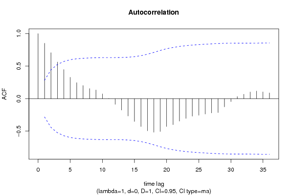
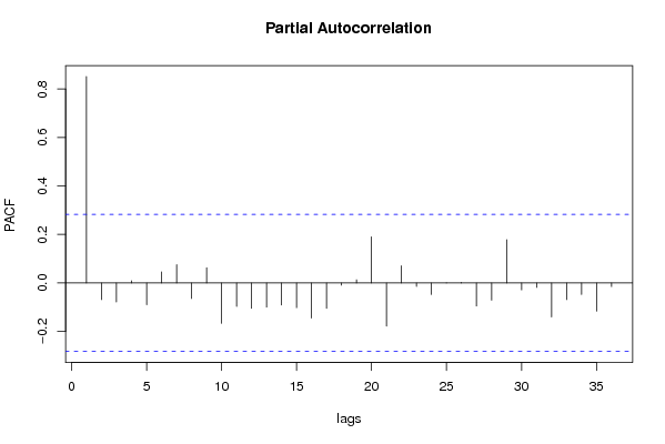
Title produced by software

(Partial) Autocorrelation Function

Date of computation

Fri, 27 Nov 2009 06:04:03 -0700

Cite this page as follows

Statistical Computations at FreeStatistics.org, Office for Research Development and Education, URL https://freestatistics.org/blog/index.php?v=date/2009/Nov/27/t12593271205n9cjg5569dh3x9.htm/, Retrieved Mon, 29 Apr 2024 18:54:22 +0000

Statistical Computations at FreeStatistics.org, Office for Research Development and Education, URL https://freestatistics.org/blog/index.php?pk=60701, Retrieved Mon, 29 Apr 2024 18:54:22 +0000

QR Codes:

Paste this QR Code to cite your computation.

Original text written by user:

IsPrivate?

No (this computation is public)

User-defined keywords

Estimated Impact

160

Family? (F = Feedback message, R = changed R code, M = changed R Module, P = changed Parameters, D = changed Data)

-     [Univariate Explorative Data Analysis] [Run Sequence gebo...] [2008-12-12 13:32:37] [76963dc1903f0f612b6153510a3818cf]
- R  D  [Univariate Explorative Data Analysis] [Run Sequence gebo...] [2008-12-17 12:14:40] [76963dc1903f0f612b6153510a3818cf]
-         [Univariate Explorative Data Analysis] [Run Sequence Plot...] [2008-12-22 18:19:51] [1ce0d16c8f4225c977b42c8fa93bc163]
- RMP       [(Partial) Autocorrelation Function] [Identifying Integ...] [2009-11-22 12:19:56] [b98453cac15ba1066b407e146608df68]
-    D          [(Partial) Autocorrelation Function] [WS 8: Methode 1 A...] [2009-11-27 13:04:03] [b9056af0304697100f456398102f1287] [Current]
-   P             [(Partial) Autocorrelation Function] [] [2009-12-05 02:26:32] [74be16979710d4c4e7c6647856088456] 

Feedback Forum

Post a new message

Dataseries X:

Download CSV

Histogram

Boxplots

Summary of computational transaction
Raw Input	view raw input (R code)
Raw Output	view raw output of R engine
Computing time	1 seconds
R Server	'Gwilym Jenkins' @ 72.249.127.135

\begin{tabular}{lllllllll}
\hline
Summary of computational transaction \tabularnewline
Raw Input & view raw input (R code)  \tabularnewline
Raw Output & view raw output of R engine  \tabularnewline
Computing time & 1 seconds \tabularnewline
R Server & 'Gwilym Jenkins' @ 72.249.127.135 \tabularnewline
\hline
\end{tabular}
%Source: https://freestatistics.org/blog/index.php?pk=60701&T=0

[TABLE]
[ROW][C]Summary of computational transaction[/C][/ROW]
[ROW][C]Raw Input[/C][C]view raw input (R code) [/C][/ROW]
[ROW][C]Raw Output[/C][C]view raw output of R engine [/C][/ROW]
[ROW][C]Computing time[/C][C]1 seconds[/C][/ROW]
[ROW][C]R Server[/C][C]'Gwilym Jenkins' @ 72.249.127.135[/C][/ROW]
[/TABLE]
Source: https://freestatistics.org/blog/index.php?pk=60701&T=0

Globally Unique Identifier (entire table): ba.freestatistics.org/blog/index.php?pk=60701&T=0

As an alternative you can also use a QR Code:

The GUIDs for individual cells are displayed in the table below:

Summary of computational transaction
Raw Input	view raw input (R code)
Raw Output	view raw output of R engine
Computing time	1 seconds
R Server	'Gwilym Jenkins' @ 72.249.127.135

Autocorrelation Function
Time lag k	ACF(k)	T-STAT	P-value
1	0.851551	5.8997	0
2	0.706251	4.893	6e-06
3	0.562739	3.8988	0.00015
4	0.446569	3.0939	0.001645
5	0.327812	2.2711	0.013831
6	0.245743	1.7026	0.047559
7	0.201334	1.3949	0.084737
8	0.154081	1.0675	0.145541
9	0.132839	0.9203	0.181001
10	0.072758	0.5041	0.308255
11	0.002283	0.0158	0.493722
12	-0.088599	-0.6138	0.271113
13	-0.17679	-1.2248	0.113307
14	-0.267568	-1.8538	0.034962
15	-0.351717	-2.4368	0.009289
16	-0.429902	-2.9784	0.002266
17	-0.495773	-3.4348	0.000616
18	-0.51687	-3.581	0.000398
19	-0.506451	-3.5088	0.000494
20	-0.429854	-2.9781	0.002268
21	-0.400513	-2.7748	0.003923
22	-0.346569	-2.4011	0.010134
23	-0.30535	-2.1155	0.0198
24	-0.27035	-1.873	0.03358
25	-0.256652	-1.7781	0.040858
26	-0.237399	-1.6448	0.053278
27	-0.220401	-1.527	0.066665
28	-0.215356	-1.492	0.071117
29	-0.12711	-0.8806	0.19145
30	-0.046463	-0.3219	0.374462
31	0.031958	0.2214	0.412855
32	0.066937	0.4638	0.32246
33	0.101583	0.7038	0.242482
34	0.116287	0.8057	0.212207
35	0.103393	0.7163	0.238631
36	0.088092	0.6103	0.272264

\begin{tabular}{lllllllll}
\hline
Autocorrelation Function \tabularnewline
Time lag k & ACF(k) & T-STAT & P-value \tabularnewline
1 & 0.851551 & 5.8997 & 0 \tabularnewline
2 & 0.706251 & 4.893 & 6e-06 \tabularnewline
3 & 0.562739 & 3.8988 & 0.00015 \tabularnewline
4 & 0.446569 & 3.0939 & 0.001645 \tabularnewline
5 & 0.327812 & 2.2711 & 0.013831 \tabularnewline
6 & 0.245743 & 1.7026 & 0.047559 \tabularnewline
7 & 0.201334 & 1.3949 & 0.084737 \tabularnewline
8 & 0.154081 & 1.0675 & 0.145541 \tabularnewline
9 & 0.132839 & 0.9203 & 0.181001 \tabularnewline
10 & 0.072758 & 0.5041 & 0.308255 \tabularnewline
11 & 0.002283 & 0.0158 & 0.493722 \tabularnewline
12 & -0.088599 & -0.6138 & 0.271113 \tabularnewline
13 & -0.17679 & -1.2248 & 0.113307 \tabularnewline
14 & -0.267568 & -1.8538 & 0.034962 \tabularnewline
15 & -0.351717 & -2.4368 & 0.009289 \tabularnewline
16 & -0.429902 & -2.9784 & 0.002266 \tabularnewline
17 & -0.495773 & -3.4348 & 0.000616 \tabularnewline
18 & -0.51687 & -3.581 & 0.000398 \tabularnewline
19 & -0.506451 & -3.5088 & 0.000494 \tabularnewline
20 & -0.429854 & -2.9781 & 0.002268 \tabularnewline
21 & -0.400513 & -2.7748 & 0.003923 \tabularnewline
22 & -0.346569 & -2.4011 & 0.010134 \tabularnewline
23 & -0.30535 & -2.1155 & 0.0198 \tabularnewline
24 & -0.27035 & -1.873 & 0.03358 \tabularnewline
25 & -0.256652 & -1.7781 & 0.040858 \tabularnewline
26 & -0.237399 & -1.6448 & 0.053278 \tabularnewline
27 & -0.220401 & -1.527 & 0.066665 \tabularnewline
28 & -0.215356 & -1.492 & 0.071117 \tabularnewline
29 & -0.12711 & -0.8806 & 0.19145 \tabularnewline
30 & -0.046463 & -0.3219 & 0.374462 \tabularnewline
31 & 0.031958 & 0.2214 & 0.412855 \tabularnewline
32 & 0.066937 & 0.4638 & 0.32246 \tabularnewline
33 & 0.101583 & 0.7038 & 0.242482 \tabularnewline
34 & 0.116287 & 0.8057 & 0.212207 \tabularnewline
35 & 0.103393 & 0.7163 & 0.238631 \tabularnewline
36 & 0.088092 & 0.6103 & 0.272264 \tabularnewline
\hline
\end{tabular}
%Source: https://freestatistics.org/blog/index.php?pk=60701&T=1

[TABLE]
[ROW][C]Autocorrelation Function[/C][/ROW]
[ROW][C]Time lag k[/C][C]ACF(k)[/C][C]T-STAT[/C][C]P-value[/C][/ROW]
[ROW][C]1[/C][C]0.851551[/C][C]5.8997[/C][C]0[/C][/ROW]
[ROW][C]2[/C][C]0.706251[/C][C]4.893[/C][C]6e-06[/C][/ROW]
[ROW][C]3[/C][C]0.562739[/C][C]3.8988[/C][C]0.00015[/C][/ROW]
[ROW][C]4[/C][C]0.446569[/C][C]3.0939[/C][C]0.001645[/C][/ROW]
[ROW][C]5[/C][C]0.327812[/C][C]2.2711[/C][C]0.013831[/C][/ROW]
[ROW][C]6[/C][C]0.245743[/C][C]1.7026[/C][C]0.047559[/C][/ROW]
[ROW][C]7[/C][C]0.201334[/C][C]1.3949[/C][C]0.084737[/C][/ROW]
[ROW][C]8[/C][C]0.154081[/C][C]1.0675[/C][C]0.145541[/C][/ROW]
[ROW][C]9[/C][C]0.132839[/C][C]0.9203[/C][C]0.181001[/C][/ROW]
[ROW][C]10[/C][C]0.072758[/C][C]0.5041[/C][C]0.308255[/C][/ROW]
[ROW][C]11[/C][C]0.002283[/C][C]0.0158[/C][C]0.493722[/C][/ROW]
[ROW][C]12[/C][C]-0.088599[/C][C]-0.6138[/C][C]0.271113[/C][/ROW]
[ROW][C]13[/C][C]-0.17679[/C][C]-1.2248[/C][C]0.113307[/C][/ROW]
[ROW][C]14[/C][C]-0.267568[/C][C]-1.8538[/C][C]0.034962[/C][/ROW]
[ROW][C]15[/C][C]-0.351717[/C][C]-2.4368[/C][C]0.009289[/C][/ROW]
[ROW][C]16[/C][C]-0.429902[/C][C]-2.9784[/C][C]0.002266[/C][/ROW]
[ROW][C]17[/C][C]-0.495773[/C][C]-3.4348[/C][C]0.000616[/C][/ROW]
[ROW][C]18[/C][C]-0.51687[/C][C]-3.581[/C][C]0.000398[/C][/ROW]
[ROW][C]19[/C][C]-0.506451[/C][C]-3.5088[/C][C]0.000494[/C][/ROW]
[ROW][C]20[/C][C]-0.429854[/C][C]-2.9781[/C][C]0.002268[/C][/ROW]
[ROW][C]21[/C][C]-0.400513[/C][C]-2.7748[/C][C]0.003923[/C][/ROW]
[ROW][C]22[/C][C]-0.346569[/C][C]-2.4011[/C][C]0.010134[/C][/ROW]
[ROW][C]23[/C][C]-0.30535[/C][C]-2.1155[/C][C]0.0198[/C][/ROW]
[ROW][C]24[/C][C]-0.27035[/C][C]-1.873[/C][C]0.03358[/C][/ROW]
[ROW][C]25[/C][C]-0.256652[/C][C]-1.7781[/C][C]0.040858[/C][/ROW]
[ROW][C]26[/C][C]-0.237399[/C][C]-1.6448[/C][C]0.053278[/C][/ROW]
[ROW][C]27[/C][C]-0.220401[/C][C]-1.527[/C][C]0.066665[/C][/ROW]
[ROW][C]28[/C][C]-0.215356[/C][C]-1.492[/C][C]0.071117[/C][/ROW]
[ROW][C]29[/C][C]-0.12711[/C][C]-0.8806[/C][C]0.19145[/C][/ROW]
[ROW][C]30[/C][C]-0.046463[/C][C]-0.3219[/C][C]0.374462[/C][/ROW]
[ROW][C]31[/C][C]0.031958[/C][C]0.2214[/C][C]0.412855[/C][/ROW]
[ROW][C]32[/C][C]0.066937[/C][C]0.4638[/C][C]0.32246[/C][/ROW]
[ROW][C]33[/C][C]0.101583[/C][C]0.7038[/C][C]0.242482[/C][/ROW]
[ROW][C]34[/C][C]0.116287[/C][C]0.8057[/C][C]0.212207[/C][/ROW]
[ROW][C]35[/C][C]0.103393[/C][C]0.7163[/C][C]0.238631[/C][/ROW]
[ROW][C]36[/C][C]0.088092[/C][C]0.6103[/C][C]0.272264[/C][/ROW]
[/TABLE]
Source: https://freestatistics.org/blog/index.php?pk=60701&T=1

Globally Unique Identifier (entire table): ba.freestatistics.org/blog/index.php?pk=60701&T=1

As an alternative you can also use a QR Code:

The GUIDs for individual cells are displayed in the table below:

Autocorrelation Function
Time lag k	ACF(k)	T-STAT	P-value
1	0.851551	5.8997	0
2	0.706251	4.893	6e-06
3	0.562739	3.8988	0.00015
4	0.446569	3.0939	0.001645
5	0.327812	2.2711	0.013831
6	0.245743	1.7026	0.047559
7	0.201334	1.3949	0.084737
8	0.154081	1.0675	0.145541
9	0.132839	0.9203	0.181001
10	0.072758	0.5041	0.308255
11	0.002283	0.0158	0.493722
12	-0.088599	-0.6138	0.271113
13	-0.17679	-1.2248	0.113307
14	-0.267568	-1.8538	0.034962
15	-0.351717	-2.4368	0.009289
16	-0.429902	-2.9784	0.002266
17	-0.495773	-3.4348	0.000616
18	-0.51687	-3.581	0.000398
19	-0.506451	-3.5088	0.000494
20	-0.429854	-2.9781	0.002268
21	-0.400513	-2.7748	0.003923
22	-0.346569	-2.4011	0.010134
23	-0.30535	-2.1155	0.0198
24	-0.27035	-1.873	0.03358
25	-0.256652	-1.7781	0.040858
26	-0.237399	-1.6448	0.053278
27	-0.220401	-1.527	0.066665
28	-0.215356	-1.492	0.071117
29	-0.12711	-0.8806	0.19145
30	-0.046463	-0.3219	0.374462
31	0.031958	0.2214	0.412855
32	0.066937	0.4638	0.32246
33	0.101583	0.7038	0.242482
34	0.116287	0.8057	0.212207
35	0.103393	0.7163	0.238631
36	0.088092	0.6103	0.272264

Partial Autocorrelation Function
Time lag k	PACF(k)	T-STAT	P-value
1	0.851551	5.8997	0
2	-0.068722	-0.4761	0.318075
3	-0.078517	-0.544	0.294486
4	0.008837	0.0612	0.475718
5	-0.089935	-0.6231	0.268089
6	0.04576	0.317	0.376296
7	0.07554	0.5234	0.301566
8	-0.064138	-0.4444	0.329389
9	0.062984	0.4364	0.332265
10	-0.166619	-1.1544	0.127032
11	-0.096833	-0.6709	0.252756
12	-0.105256	-0.7292	0.234701
13	-0.099796	-0.6914	0.24632
14	-0.091196	-0.6318	0.26525
15	-0.1021	-0.7074	0.241379
16	-0.145084	-1.0052	0.159928
17	-0.105122	-0.7283	0.234982
18	-0.009538	-0.0661	0.473794
19	0.012828	0.0889	0.464776
20	0.190113	1.3171	0.097022
21	-0.178082	-1.2338	0.111645
22	0.070723	0.49	0.313189
23	-0.014463	-0.1002	0.4603
24	-0.047811	-0.3312	0.37095
25	0.000517	0.0036	0.498577
26	0.002011	0.0139	0.494471
27	-0.095107	-0.6589	0.256549
28	-0.071177	-0.4931	0.312085
29	0.178469	1.2365	0.111151
30	-0.028857	-0.1999	0.421192
31	-0.018625	-0.129	0.448935
32	-0.1406	-0.9741	0.167444
33	-0.06893	-0.4776	0.317566
34	-0.047616	-0.3299	0.371457
35	-0.116524	-0.8073	0.211737
36	-0.015247	-0.1056	0.458156

\begin{tabular}{lllllllll}
\hline
Partial Autocorrelation Function \tabularnewline
Time lag k & PACF(k) & T-STAT & P-value \tabularnewline
1 & 0.851551 & 5.8997 & 0 \tabularnewline
2 & -0.068722 & -0.4761 & 0.318075 \tabularnewline
3 & -0.078517 & -0.544 & 0.294486 \tabularnewline
4 & 0.008837 & 0.0612 & 0.475718 \tabularnewline
5 & -0.089935 & -0.6231 & 0.268089 \tabularnewline
6 & 0.04576 & 0.317 & 0.376296 \tabularnewline
7 & 0.07554 & 0.5234 & 0.301566 \tabularnewline
8 & -0.064138 & -0.4444 & 0.329389 \tabularnewline
9 & 0.062984 & 0.4364 & 0.332265 \tabularnewline
10 & -0.166619 & -1.1544 & 0.127032 \tabularnewline
11 & -0.096833 & -0.6709 & 0.252756 \tabularnewline
12 & -0.105256 & -0.7292 & 0.234701 \tabularnewline
13 & -0.099796 & -0.6914 & 0.24632 \tabularnewline
14 & -0.091196 & -0.6318 & 0.26525 \tabularnewline
15 & -0.1021 & -0.7074 & 0.241379 \tabularnewline
16 & -0.145084 & -1.0052 & 0.159928 \tabularnewline
17 & -0.105122 & -0.7283 & 0.234982 \tabularnewline
18 & -0.009538 & -0.0661 & 0.473794 \tabularnewline
19 & 0.012828 & 0.0889 & 0.464776 \tabularnewline
20 & 0.190113 & 1.3171 & 0.097022 \tabularnewline
21 & -0.178082 & -1.2338 & 0.111645 \tabularnewline
22 & 0.070723 & 0.49 & 0.313189 \tabularnewline
23 & -0.014463 & -0.1002 & 0.4603 \tabularnewline
24 & -0.047811 & -0.3312 & 0.37095 \tabularnewline
25 & 0.000517 & 0.0036 & 0.498577 \tabularnewline
26 & 0.002011 & 0.0139 & 0.494471 \tabularnewline
27 & -0.095107 & -0.6589 & 0.256549 \tabularnewline
28 & -0.071177 & -0.4931 & 0.312085 \tabularnewline
29 & 0.178469 & 1.2365 & 0.111151 \tabularnewline
30 & -0.028857 & -0.1999 & 0.421192 \tabularnewline
31 & -0.018625 & -0.129 & 0.448935 \tabularnewline
32 & -0.1406 & -0.9741 & 0.167444 \tabularnewline
33 & -0.06893 & -0.4776 & 0.317566 \tabularnewline
34 & -0.047616 & -0.3299 & 0.371457 \tabularnewline
35 & -0.116524 & -0.8073 & 0.211737 \tabularnewline
36 & -0.015247 & -0.1056 & 0.458156 \tabularnewline
\hline
\end{tabular}
%Source: https://freestatistics.org/blog/index.php?pk=60701&T=2

[TABLE]
[ROW][C]Partial Autocorrelation Function[/C][/ROW]
[ROW][C]Time lag k[/C][C]PACF(k)[/C][C]T-STAT[/C][C]P-value[/C][/ROW]
[ROW][C]1[/C][C]0.851551[/C][C]5.8997[/C][C]0[/C][/ROW]
[ROW][C]2[/C][C]-0.068722[/C][C]-0.4761[/C][C]0.318075[/C][/ROW]
[ROW][C]3[/C][C]-0.078517[/C][C]-0.544[/C][C]0.294486[/C][/ROW]
[ROW][C]4[/C][C]0.008837[/C][C]0.0612[/C][C]0.475718[/C][/ROW]
[ROW][C]5[/C][C]-0.089935[/C][C]-0.6231[/C][C]0.268089[/C][/ROW]
[ROW][C]6[/C][C]0.04576[/C][C]0.317[/C][C]0.376296[/C][/ROW]
[ROW][C]7[/C][C]0.07554[/C][C]0.5234[/C][C]0.301566[/C][/ROW]
[ROW][C]8[/C][C]-0.064138[/C][C]-0.4444[/C][C]0.329389[/C][/ROW]
[ROW][C]9[/C][C]0.062984[/C][C]0.4364[/C][C]0.332265[/C][/ROW]
[ROW][C]10[/C][C]-0.166619[/C][C]-1.1544[/C][C]0.127032[/C][/ROW]
[ROW][C]11[/C][C]-0.096833[/C][C]-0.6709[/C][C]0.252756[/C][/ROW]
[ROW][C]12[/C][C]-0.105256[/C][C]-0.7292[/C][C]0.234701[/C][/ROW]
[ROW][C]13[/C][C]-0.099796[/C][C]-0.6914[/C][C]0.24632[/C][/ROW]
[ROW][C]14[/C][C]-0.091196[/C][C]-0.6318[/C][C]0.26525[/C][/ROW]
[ROW][C]15[/C][C]-0.1021[/C][C]-0.7074[/C][C]0.241379[/C][/ROW]
[ROW][C]16[/C][C]-0.145084[/C][C]-1.0052[/C][C]0.159928[/C][/ROW]
[ROW][C]17[/C][C]-0.105122[/C][C]-0.7283[/C][C]0.234982[/C][/ROW]
[ROW][C]18[/C][C]-0.009538[/C][C]-0.0661[/C][C]0.473794[/C][/ROW]
[ROW][C]19[/C][C]0.012828[/C][C]0.0889[/C][C]0.464776[/C][/ROW]
[ROW][C]20[/C][C]0.190113[/C][C]1.3171[/C][C]0.097022[/C][/ROW]
[ROW][C]21[/C][C]-0.178082[/C][C]-1.2338[/C][C]0.111645[/C][/ROW]
[ROW][C]22[/C][C]0.070723[/C][C]0.49[/C][C]0.313189[/C][/ROW]
[ROW][C]23[/C][C]-0.014463[/C][C]-0.1002[/C][C]0.4603[/C][/ROW]
[ROW][C]24[/C][C]-0.047811[/C][C]-0.3312[/C][C]0.37095[/C][/ROW]
[ROW][C]25[/C][C]0.000517[/C][C]0.0036[/C][C]0.498577[/C][/ROW]
[ROW][C]26[/C][C]0.002011[/C][C]0.0139[/C][C]0.494471[/C][/ROW]
[ROW][C]27[/C][C]-0.095107[/C][C]-0.6589[/C][C]0.256549[/C][/ROW]
[ROW][C]28[/C][C]-0.071177[/C][C]-0.4931[/C][C]0.312085[/C][/ROW]
[ROW][C]29[/C][C]0.178469[/C][C]1.2365[/C][C]0.111151[/C][/ROW]
[ROW][C]30[/C][C]-0.028857[/C][C]-0.1999[/C][C]0.421192[/C][/ROW]
[ROW][C]31[/C][C]-0.018625[/C][C]-0.129[/C][C]0.448935[/C][/ROW]
[ROW][C]32[/C][C]-0.1406[/C][C]-0.9741[/C][C]0.167444[/C][/ROW]
[ROW][C]33[/C][C]-0.06893[/C][C]-0.4776[/C][C]0.317566[/C][/ROW]
[ROW][C]34[/C][C]-0.047616[/C][C]-0.3299[/C][C]0.371457[/C][/ROW]
[ROW][C]35[/C][C]-0.116524[/C][C]-0.8073[/C][C]0.211737[/C][/ROW]
[ROW][C]36[/C][C]-0.015247[/C][C]-0.1056[/C][C]0.458156[/C][/ROW]
[/TABLE]
Source: https://freestatistics.org/blog/index.php?pk=60701&T=2

Globally Unique Identifier (entire table): ba.freestatistics.org/blog/index.php?pk=60701&T=2

As an alternative you can also use a QR Code:

The GUIDs for individual cells are displayed in the table below:

Partial Autocorrelation Function
Time lag k	PACF(k)	T-STAT	P-value
1	0.851551	5.8997	0
2	-0.068722	-0.4761	0.318075
3	-0.078517	-0.544	0.294486
4	0.008837	0.0612	0.475718
5	-0.089935	-0.6231	0.268089
6	0.04576	0.317	0.376296
7	0.07554	0.5234	0.301566
8	-0.064138	-0.4444	0.329389
9	0.062984	0.4364	0.332265
10	-0.166619	-1.1544	0.127032
11	-0.096833	-0.6709	0.252756
12	-0.105256	-0.7292	0.234701
13	-0.099796	-0.6914	0.24632
14	-0.091196	-0.6318	0.26525
15	-0.1021	-0.7074	0.241379
16	-0.145084	-1.0052	0.159928
17	-0.105122	-0.7283	0.234982
18	-0.009538	-0.0661	0.473794
19	0.012828	0.0889	0.464776
20	0.190113	1.3171	0.097022
21	-0.178082	-1.2338	0.111645
22	0.070723	0.49	0.313189
23	-0.014463	-0.1002	0.4603
24	-0.047811	-0.3312	0.37095
25	0.000517	0.0036	0.498577
26	0.002011	0.0139	0.494471
27	-0.095107	-0.6589	0.256549
28	-0.071177	-0.4931	0.312085
29	0.178469	1.2365	0.111151
30	-0.028857	-0.1999	0.421192
31	-0.018625	-0.129	0.448935
32	-0.1406	-0.9741	0.167444
33	-0.06893	-0.4776	0.317566
34	-0.047616	-0.3299	0.371457
35	-0.116524	-0.8073	0.211737
36	-0.015247	-0.1056	0.458156

Figure 1

PNG link

Postscript link

PDF link

Figure 2

PNG link

Postscript link

PDF link

Parameters (Session):

par1 = 36 ; par2 = 1 ; par3 = 0 ; par4 = 1 ; par5 = 12 ; par6 = MA ; par7 = 0.95 ;

Parameters (R input):

par1 = 36 ; par2 = 1 ; par3 = 0 ; par4 = 1 ; par5 = 12 ; par6 = MA ; par7 = 0.95 ;

R code (references can be found in the software module):

if (par1 == 'Default') {
par1 = 10*log10(length(x))
} else {
par1 <- as.numeric(par1)
}
par2 <- as.numeric(par2)
par3 <- as.numeric(par3)
par4 <- as.numeric(par4)
par5 <- as.numeric(par5)
if (par6 == 'White Noise') par6 <- 'white' else par6 <- 'ma'
par7 <- as.numeric(par7)
if (par2 == 0) {
x <- log(x)
} else {
x <- (x ^ par2 - 1) / par2
}
if (par3 > 0) x <- diff(x,lag=1,difference=par3)
if (par4 > 0) x <- diff(x,lag=par5,difference=par4)
bitmap(file='pic1.png')
racf <- acf(x, par1, main='Autocorrelation', xlab='time lag', ylab='ACF', ci.type=par6, ci=par7, sub=paste('(lambda=',par2,', d=',par3,', D=',par4,', CI=', par7, ', CI type=',par6,')',sep=''))
dev.off()
bitmap(file='pic2.png')
rpacf <- pacf(x,par1,main='Partial Autocorrelation',xlab='lags',ylab='PACF')
dev.off()
(myacf <- c(racf$acf))
(mypacf <- c(rpacf$acf))
lengthx <- length(x)
sqrtn <- sqrt(lengthx)
load(file='createtable')
a<-table.start()
a<-table.row.start(a)
a<-table.element(a,'Autocorrelation Function',4,TRUE)
a<-table.row.end(a)
a<-table.row.start(a)
a<-table.element(a,'Time lag k',header=TRUE)
a<-table.element(a,hyperlink('basics.htm','ACF(k)','click here for more information about the Autocorrelation Function'),header=TRUE)
a<-table.element(a,'T-STAT',header=TRUE)
a<-table.element(a,'P-value',header=TRUE)
a<-table.row.end(a)
for (i in 2:(par1+1)) {
a<-table.row.start(a)
a<-table.element(a,i-1,header=TRUE)
a<-table.element(a,round(myacf[i],6))
mytstat <- myacf[i]*sqrtn
a<-table.element(a,round(mytstat,4))
a<-table.element(a,round(1-pt(abs(mytstat),lengthx),6))
a<-table.row.end(a)
}
a<-table.end(a)
table.save(a,file='mytable.tab')
a<-table.start()
a<-table.row.start(a)
a<-table.element(a,'Partial Autocorrelation Function',4,TRUE)
a<-table.row.end(a)
a<-table.row.start(a)
a<-table.element(a,'Time lag k',header=TRUE)
a<-table.element(a,hyperlink('basics.htm','PACF(k)','click here for more information about the Partial Autocorrelation Function'),header=TRUE)
a<-table.element(a,'T-STAT',header=TRUE)
a<-table.element(a,'P-value',header=TRUE)
a<-table.row.end(a)
for (i in 1:par1) {
a<-table.row.start(a)
a<-table.element(a,i,header=TRUE)
a<-table.element(a,round(mypacf[i],6))
mytstat <- mypacf[i]*sqrtn
a<-table.element(a,round(mytstat,4))
a<-table.element(a,round(1-pt(abs(mytstat),lengthx),6))
a<-table.row.end(a)
}
a<-table.end(a)
table.save(a,file='mytable1.tab')

Free Statistics

Description of Statistical Computation

Tree of Dependent Computations

Dataset

Tables (Output of Computation)

Figures (Output of Computation)

Input Parameters & R Code