Repository of Reproducible Computations

Free Statistics

of Irreproducible Research!

Author's title

Author

*The author of this computation has been verified*

R Software Module

rwasp_autocorrelation.wasp

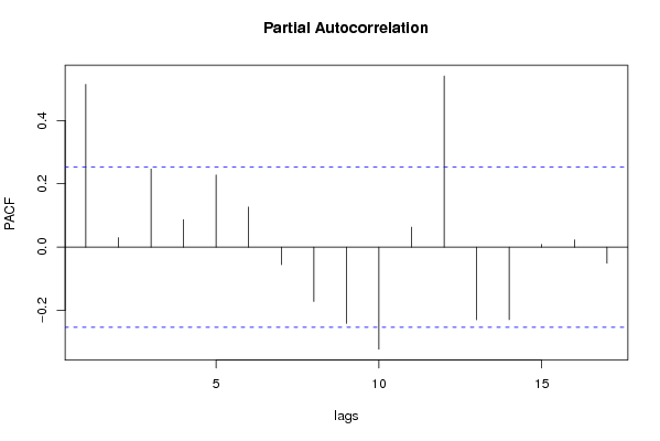
Title produced by software

(Partial) Autocorrelation Function

Date of computation

Wed, 25 Nov 2009 13:17:41 -0700

Cite this page as follows

Statistical Computations at FreeStatistics.org, Office for Research Development and Education, URL https://freestatistics.org/blog/index.php?v=date/2009/Nov/25/t125918032157pv1uquod1vuj6.htm/, Retrieved Wed, 08 May 2024 13:59:40 +0000

Statistical Computations at FreeStatistics.org, Office for Research Development and Education, URL https://freestatistics.org/blog/index.php?pk=59609, Retrieved Wed, 08 May 2024 13:59:40 +0000

QR Codes:

Paste this QR Code to cite your computation.

Original text written by user:

IsPrivate?

No (this computation is public)

User-defined keywords

Estimated Impact

175

Family? (F = Feedback message, R = changed R code, M = changed R Module, P = changed Parameters, D = changed Data)

F       [(Partial) Autocorrelation Function] [acf methode] [2009-11-25 20:17:41] [bef26de542bed2eafc60fe4615b06e47] [Current]
-   P     [(Partial) Autocorrelation Function] [acf methode] [2009-11-30 18:48:24] [21324e9cdf3569788a3d630236984d87] 
-   P     [(Partial) Autocorrelation Function] [acf methode] [2009-11-30 18:50:07] [21324e9cdf3569788a3d630236984d87] 
-    D      [(Partial) Autocorrelation Function] [] [2010-12-16 14:40:12] [f47feae0308dca73181bb669fbad1c56] 
-   PD        [(Partial) Autocorrelation Function] [] [2010-12-16 14:50:06] [f47feae0308dca73181bb669fbad1c56] 
-   P           [(Partial) Autocorrelation Function] [] [2010-12-20 09:18:41] [f47feae0308dca73181bb669fbad1c56] 
-   P           [(Partial) Autocorrelation Function] [] [2010-12-20 09:30:33] [f47feae0308dca73181bb669fbad1c56] 
-   P           [(Partial) Autocorrelation Function] [] [2010-12-20 09:36:47] [f47feae0308dca73181bb669fbad1c56] 
-   P     [(Partial) Autocorrelation Function] [acf methode] [2009-11-30 18:54:14] [21324e9cdf3569788a3d630236984d87] 
-    D      [(Partial) Autocorrelation Function] [] [2010-12-16 14:55:48] [f47feae0308dca73181bb669fbad1c56] 
-   P     [(Partial) Autocorrelation Function] [acf methode] [2009-11-30 18:55:57] [21324e9cdf3569788a3d630236984d87] 

Feedback Forum

2009-11-26 09:15:25 [] [reply] 
is het mogelijk om beschrijving en een naam te geven van de tijdreeks? ik weet niet over wat het gaat> 
in de tabel van de eerste link gaan de waarden maar tot 17. 
bij de number of time lags moet je 36 invullen en bij CI type: MA 
ook bemerk ik een outlier in de twaalfde maand met een lage p-waarde, dus hoge correlatie en niet door toeval. ik zie op deze grafiek dus enkel tot maand 17  

Post a new message

Dataseries X:

Download CSV

Histogram

Boxplots

Summary of computational transaction
Raw Input	view raw input (R code)
Raw Output	view raw output of R engine
Computing time	2 seconds
R Server	'Gwilym Jenkins' @ 72.249.127.135

\begin{tabular}{lllllllll}
\hline
Summary of computational transaction \tabularnewline
Raw Input & view raw input (R code)  \tabularnewline
Raw Output & view raw output of R engine  \tabularnewline
Computing time & 2 seconds \tabularnewline
R Server & 'Gwilym Jenkins' @ 72.249.127.135 \tabularnewline
\hline
\end{tabular}
%Source: https://freestatistics.org/blog/index.php?pk=59609&T=0

[TABLE]
[ROW][C]Summary of computational transaction[/C][/ROW]
[ROW][C]Raw Input[/C][C]view raw input (R code) [/C][/ROW]
[ROW][C]Raw Output[/C][C]view raw output of R engine [/C][/ROW]
[ROW][C]Computing time[/C][C]2 seconds[/C][/ROW]
[ROW][C]R Server[/C][C]'Gwilym Jenkins' @ 72.249.127.135[/C][/ROW]
[/TABLE]
Source: https://freestatistics.org/blog/index.php?pk=59609&T=0

Globally Unique Identifier (entire table): ba.freestatistics.org/blog/index.php?pk=59609&T=0

As an alternative you can also use a QR Code:

The GUIDs for individual cells are displayed in the table below:

Summary of computational transaction
Raw Input	view raw input (R code)
Raw Output	view raw output of R engine
Computing time	2 seconds
R Server	'Gwilym Jenkins' @ 72.249.127.135

Autocorrelation Function
Time lag k	ACF(k)	T-STAT	P-value
1	0.514089	3.9821	9.4e-05
2	0.286353	2.2181	0.015173
3	0.339561	2.6302	0.005413
4	0.327069	2.5335	0.006962
5	0.38416	2.9757	0.002104
6	0.399257	3.0926	0.001505
7	0.259675	2.0114	0.024389
8	0.101437	0.7857	0.217558
9	-0.013223	-0.1024	0.459382
10	-0.122561	-0.9494	0.173124
11	0.027485	0.2129	0.416063
12	0.33501	2.595	0.005937
13	-0.010602	-0.0821	0.467412
14	-0.256963	-1.9904	0.025553
15	-0.158708	-1.2293	0.11187
16	-0.130946	-1.0143	0.157256
17	-0.063386	-0.491	0.312614

\begin{tabular}{lllllllll}
\hline
Autocorrelation Function \tabularnewline
Time lag k & ACF(k) & T-STAT & P-value \tabularnewline
1 & 0.514089 & 3.9821 & 9.4e-05 \tabularnewline
2 & 0.286353 & 2.2181 & 0.015173 \tabularnewline
3 & 0.339561 & 2.6302 & 0.005413 \tabularnewline
4 & 0.327069 & 2.5335 & 0.006962 \tabularnewline
5 & 0.38416 & 2.9757 & 0.002104 \tabularnewline
6 & 0.399257 & 3.0926 & 0.001505 \tabularnewline
7 & 0.259675 & 2.0114 & 0.024389 \tabularnewline
8 & 0.101437 & 0.7857 & 0.217558 \tabularnewline
9 & -0.013223 & -0.1024 & 0.459382 \tabularnewline
10 & -0.122561 & -0.9494 & 0.173124 \tabularnewline
11 & 0.027485 & 0.2129 & 0.416063 \tabularnewline
12 & 0.33501 & 2.595 & 0.005937 \tabularnewline
13 & -0.010602 & -0.0821 & 0.467412 \tabularnewline
14 & -0.256963 & -1.9904 & 0.025553 \tabularnewline
15 & -0.158708 & -1.2293 & 0.11187 \tabularnewline
16 & -0.130946 & -1.0143 & 0.157256 \tabularnewline
17 & -0.063386 & -0.491 & 0.312614 \tabularnewline
\hline
\end{tabular}
%Source: https://freestatistics.org/blog/index.php?pk=59609&T=1

[TABLE]
[ROW][C]Autocorrelation Function[/C][/ROW]
[ROW][C]Time lag k[/C][C]ACF(k)[/C][C]T-STAT[/C][C]P-value[/C][/ROW]
[ROW][C]1[/C][C]0.514089[/C][C]3.9821[/C][C]9.4e-05[/C][/ROW]
[ROW][C]2[/C][C]0.286353[/C][C]2.2181[/C][C]0.015173[/C][/ROW]
[ROW][C]3[/C][C]0.339561[/C][C]2.6302[/C][C]0.005413[/C][/ROW]
[ROW][C]4[/C][C]0.327069[/C][C]2.5335[/C][C]0.006962[/C][/ROW]
[ROW][C]5[/C][C]0.38416[/C][C]2.9757[/C][C]0.002104[/C][/ROW]
[ROW][C]6[/C][C]0.399257[/C][C]3.0926[/C][C]0.001505[/C][/ROW]
[ROW][C]7[/C][C]0.259675[/C][C]2.0114[/C][C]0.024389[/C][/ROW]
[ROW][C]8[/C][C]0.101437[/C][C]0.7857[/C][C]0.217558[/C][/ROW]
[ROW][C]9[/C][C]-0.013223[/C][C]-0.1024[/C][C]0.459382[/C][/ROW]
[ROW][C]10[/C][C]-0.122561[/C][C]-0.9494[/C][C]0.173124[/C][/ROW]
[ROW][C]11[/C][C]0.027485[/C][C]0.2129[/C][C]0.416063[/C][/ROW]
[ROW][C]12[/C][C]0.33501[/C][C]2.595[/C][C]0.005937[/C][/ROW]
[ROW][C]13[/C][C]-0.010602[/C][C]-0.0821[/C][C]0.467412[/C][/ROW]
[ROW][C]14[/C][C]-0.256963[/C][C]-1.9904[/C][C]0.025553[/C][/ROW]
[ROW][C]15[/C][C]-0.158708[/C][C]-1.2293[/C][C]0.11187[/C][/ROW]
[ROW][C]16[/C][C]-0.130946[/C][C]-1.0143[/C][C]0.157256[/C][/ROW]
[ROW][C]17[/C][C]-0.063386[/C][C]-0.491[/C][C]0.312614[/C][/ROW]
[/TABLE]
Source: https://freestatistics.org/blog/index.php?pk=59609&T=1

Globally Unique Identifier (entire table): ba.freestatistics.org/blog/index.php?pk=59609&T=1

As an alternative you can also use a QR Code:

The GUIDs for individual cells are displayed in the table below:

Autocorrelation Function
Time lag k	ACF(k)	T-STAT	P-value
1	0.514089	3.9821	9.4e-05
2	0.286353	2.2181	0.015173
3	0.339561	2.6302	0.005413
4	0.327069	2.5335	0.006962
5	0.38416	2.9757	0.002104
6	0.399257	3.0926	0.001505
7	0.259675	2.0114	0.024389
8	0.101437	0.7857	0.217558
9	-0.013223	-0.1024	0.459382
10	-0.122561	-0.9494	0.173124
11	0.027485	0.2129	0.416063
12	0.33501	2.595	0.005937
13	-0.010602	-0.0821	0.467412
14	-0.256963	-1.9904	0.025553
15	-0.158708	-1.2293	0.11187
16	-0.130946	-1.0143	0.157256
17	-0.063386	-0.491	0.312614

Partial Autocorrelation Function
Time lag k	PACF(k)	T-STAT	P-value
1	0.514089	3.9821	9.4e-05
2	0.029991	0.2323	0.408543
3	0.246713	1.911	0.030391
4	0.087006	0.6739	0.251468
5	0.228013	1.7662	0.041226
6	0.126405	0.9791	0.165725
7	-0.055646	-0.431	0.333996
8	-0.171624	-1.3294	0.094375
9	-0.241126	-1.8678	0.033341
10	-0.322286	-2.4964	0.007655
11	0.063175	0.4894	0.313187
12	0.540671	4.188	4.7e-05
13	-0.229463	-1.7774	0.040285
14	-0.229359	-1.7766	0.040351
15	0.008563	0.0663	0.473668
16	0.022862	0.1771	0.430019
17	-0.050683	-0.3926	0.348008

\begin{tabular}{lllllllll}
\hline
Partial Autocorrelation Function \tabularnewline
Time lag k & PACF(k) & T-STAT & P-value \tabularnewline
1 & 0.514089 & 3.9821 & 9.4e-05 \tabularnewline
2 & 0.029991 & 0.2323 & 0.408543 \tabularnewline
3 & 0.246713 & 1.911 & 0.030391 \tabularnewline
4 & 0.087006 & 0.6739 & 0.251468 \tabularnewline
5 & 0.228013 & 1.7662 & 0.041226 \tabularnewline
6 & 0.126405 & 0.9791 & 0.165725 \tabularnewline
7 & -0.055646 & -0.431 & 0.333996 \tabularnewline
8 & -0.171624 & -1.3294 & 0.094375 \tabularnewline
9 & -0.241126 & -1.8678 & 0.033341 \tabularnewline
10 & -0.322286 & -2.4964 & 0.007655 \tabularnewline
11 & 0.063175 & 0.4894 & 0.313187 \tabularnewline
12 & 0.540671 & 4.188 & 4.7e-05 \tabularnewline
13 & -0.229463 & -1.7774 & 0.040285 \tabularnewline
14 & -0.229359 & -1.7766 & 0.040351 \tabularnewline
15 & 0.008563 & 0.0663 & 0.473668 \tabularnewline
16 & 0.022862 & 0.1771 & 0.430019 \tabularnewline
17 & -0.050683 & -0.3926 & 0.348008 \tabularnewline
\hline
\end{tabular}
%Source: https://freestatistics.org/blog/index.php?pk=59609&T=2

[TABLE]
[ROW][C]Partial Autocorrelation Function[/C][/ROW]
[ROW][C]Time lag k[/C][C]PACF(k)[/C][C]T-STAT[/C][C]P-value[/C][/ROW]
[ROW][C]1[/C][C]0.514089[/C][C]3.9821[/C][C]9.4e-05[/C][/ROW]
[ROW][C]2[/C][C]0.029991[/C][C]0.2323[/C][C]0.408543[/C][/ROW]
[ROW][C]3[/C][C]0.246713[/C][C]1.911[/C][C]0.030391[/C][/ROW]
[ROW][C]4[/C][C]0.087006[/C][C]0.6739[/C][C]0.251468[/C][/ROW]
[ROW][C]5[/C][C]0.228013[/C][C]1.7662[/C][C]0.041226[/C][/ROW]
[ROW][C]6[/C][C]0.126405[/C][C]0.9791[/C][C]0.165725[/C][/ROW]
[ROW][C]7[/C][C]-0.055646[/C][C]-0.431[/C][C]0.333996[/C][/ROW]
[ROW][C]8[/C][C]-0.171624[/C][C]-1.3294[/C][C]0.094375[/C][/ROW]
[ROW][C]9[/C][C]-0.241126[/C][C]-1.8678[/C][C]0.033341[/C][/ROW]
[ROW][C]10[/C][C]-0.322286[/C][C]-2.4964[/C][C]0.007655[/C][/ROW]
[ROW][C]11[/C][C]0.063175[/C][C]0.4894[/C][C]0.313187[/C][/ROW]
[ROW][C]12[/C][C]0.540671[/C][C]4.188[/C][C]4.7e-05[/C][/ROW]
[ROW][C]13[/C][C]-0.229463[/C][C]-1.7774[/C][C]0.040285[/C][/ROW]
[ROW][C]14[/C][C]-0.229359[/C][C]-1.7766[/C][C]0.040351[/C][/ROW]
[ROW][C]15[/C][C]0.008563[/C][C]0.0663[/C][C]0.473668[/C][/ROW]
[ROW][C]16[/C][C]0.022862[/C][C]0.1771[/C][C]0.430019[/C][/ROW]
[ROW][C]17[/C][C]-0.050683[/C][C]-0.3926[/C][C]0.348008[/C][/ROW]
[/TABLE]
Source: https://freestatistics.org/blog/index.php?pk=59609&T=2

Globally Unique Identifier (entire table): ba.freestatistics.org/blog/index.php?pk=59609&T=2

As an alternative you can also use a QR Code:

The GUIDs for individual cells are displayed in the table below:

Partial Autocorrelation Function
Time lag k	PACF(k)	T-STAT	P-value
1	0.514089	3.9821	9.4e-05
2	0.029991	0.2323	0.408543
3	0.246713	1.911	0.030391
4	0.087006	0.6739	0.251468
5	0.228013	1.7662	0.041226
6	0.126405	0.9791	0.165725
7	-0.055646	-0.431	0.333996
8	-0.171624	-1.3294	0.094375
9	-0.241126	-1.8678	0.033341
10	-0.322286	-2.4964	0.007655
11	0.063175	0.4894	0.313187
12	0.540671	4.188	4.7e-05
13	-0.229463	-1.7774	0.040285
14	-0.229359	-1.7766	0.040351
15	0.008563	0.0663	0.473668
16	0.022862	0.1771	0.430019
17	-0.050683	-0.3926	0.348008

Figure 1

PNG link

Postscript link

PDF link

Figure 2

PNG link

Postscript link

PDF link

Parameters (Session):

par1 = Default ; par2 = 1 ; par3 = 0 ; par4 = 0 ; par5 = 12 ; par6 = White Noise ; par7 = 0.95 ;

Parameters (R input):

par1 = Default ; par2 = 1 ; par3 = 0 ; par4 = 0 ; par5 = 12 ; par6 = White Noise ; par7 = 0.95 ;

R code (references can be found in the software module):

if (par1 == 'Default') {
par1 = 10*log10(length(x))
} else {
par1 <- as.numeric(par1)
}
par2 <- as.numeric(par2)
par3 <- as.numeric(par3)
par4 <- as.numeric(par4)
par5 <- as.numeric(par5)
if (par6 == 'White Noise') par6 <- 'white' else par6 <- 'ma'
par7 <- as.numeric(par7)
if (par2 == 0) {
x <- log(x)
} else {
x <- (x ^ par2 - 1) / par2
}
if (par3 > 0) x <- diff(x,lag=1,difference=par3)
if (par4 > 0) x <- diff(x,lag=par5,difference=par4)
bitmap(file='pic1.png')
racf <- acf(x, par1, main='Autocorrelation', xlab='time lag', ylab='ACF', ci.type=par6, ci=par7, sub=paste('(lambda=',par2,', d=',par3,', D=',par4,', CI=', par7, ', CI type=',par6,')',sep=''))
dev.off()
bitmap(file='pic2.png')
rpacf <- pacf(x,par1,main='Partial Autocorrelation',xlab='lags',ylab='PACF')
dev.off()
(myacf <- c(racf$acf))
(mypacf <- c(rpacf$acf))
lengthx <- length(x)
sqrtn <- sqrt(lengthx)
load(file='createtable')
a<-table.start()
a<-table.row.start(a)
a<-table.element(a,'Autocorrelation Function',4,TRUE)
a<-table.row.end(a)
a<-table.row.start(a)
a<-table.element(a,'Time lag k',header=TRUE)
a<-table.element(a,hyperlink('basics.htm','ACF(k)','click here for more information about the Autocorrelation Function'),header=TRUE)
a<-table.element(a,'T-STAT',header=TRUE)
a<-table.element(a,'P-value',header=TRUE)
a<-table.row.end(a)
for (i in 2:(par1+1)) {
a<-table.row.start(a)
a<-table.element(a,i-1,header=TRUE)
a<-table.element(a,round(myacf[i],6))
mytstat <- myacf[i]*sqrtn
a<-table.element(a,round(mytstat,4))
a<-table.element(a,round(1-pt(abs(mytstat),lengthx),6))
a<-table.row.end(a)
}
a<-table.end(a)
table.save(a,file='mytable.tab')
a<-table.start()
a<-table.row.start(a)
a<-table.element(a,'Partial Autocorrelation Function',4,TRUE)
a<-table.row.end(a)
a<-table.row.start(a)
a<-table.element(a,'Time lag k',header=TRUE)
a<-table.element(a,hyperlink('basics.htm','PACF(k)','click here for more information about the Partial Autocorrelation Function'),header=TRUE)
a<-table.element(a,'T-STAT',header=TRUE)
a<-table.element(a,'P-value',header=TRUE)
a<-table.row.end(a)
for (i in 1:par1) {
a<-table.row.start(a)
a<-table.element(a,i,header=TRUE)
a<-table.element(a,round(mypacf[i],6))
mytstat <- mypacf[i]*sqrtn
a<-table.element(a,round(mytstat,4))
a<-table.element(a,round(1-pt(abs(mytstat),lengthx),6))
a<-table.row.end(a)
}
a<-table.end(a)
table.save(a,file='mytable1.tab')

Free Statistics

Description of Statistical Computation

Tree of Dependent Computations

Dataset

Tables (Output of Computation)

Figures (Output of Computation)

Input Parameters & R Code