Repository of Reproducible Computations

Free Statistics

of Irreproducible Research!

Author's title

Author

*The author of this computation has been verified*

R Software Module

rwasp_autocorrelation.wasp

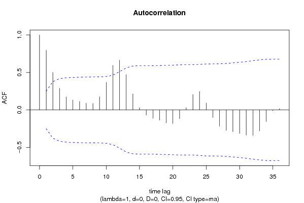
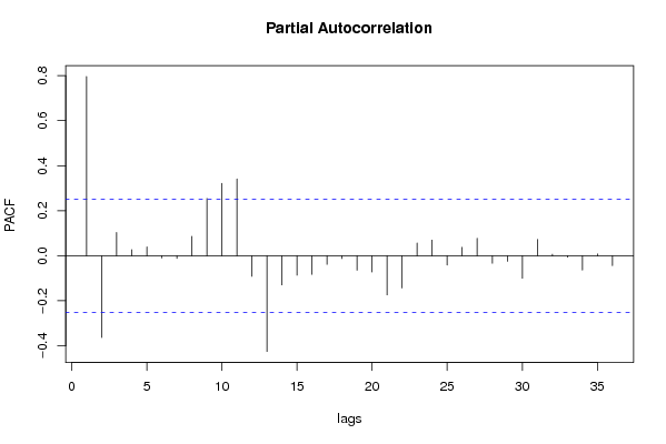
Title produced by software

(Partial) Autocorrelation Function

Date of computation

Tue, 24 Nov 2009 11:19:05 -0700

Cite this page as follows

Statistical Computations at FreeStatistics.org, Office for Research Development and Education, URL https://freestatistics.org/blog/index.php?v=date/2009/Nov/24/t1259086806kmr1inhf1apyira.htm/, Retrieved Wed, 24 Apr 2024 22:27:31 +0000

Statistical Computations at FreeStatistics.org, Office for Research Development and Education, URL https://freestatistics.org/blog/index.php?pk=59203, Retrieved Wed, 24 Apr 2024 22:27:31 +0000

QR Codes:

Paste this QR Code to cite your computation.

Original text written by user:

IsPrivate?

No (this computation is public)

User-defined keywords

Workshop 8 - methode 1 link 1

Estimated Impact

144

Family? (F = Feedback message, R = changed R code, M = changed R Module, P = changed Parameters, D = changed Data)

-     [Univariate Explorative Data Analysis] [Run Sequence gebo...] [2008-12-12 13:32:37] [76963dc1903f0f612b6153510a3818cf]
- R  D  [Univariate Explorative Data Analysis] [Run Sequence gebo...] [2008-12-17 12:14:40] [76963dc1903f0f612b6153510a3818cf]
-         [Univariate Explorative Data Analysis] [Run Sequence Plot...] [2008-12-22 18:19:51] [1ce0d16c8f4225c977b42c8fa93bc163]
- RMP       [(Partial) Autocorrelation Function] [Identifying Integ...] [2009-11-22 12:16:10] [b98453cac15ba1066b407e146608df68]
-    D          [(Partial) Autocorrelation Function] [Workshop 8] [2009-11-24 18:19:05] [100339cefec36dfa6f2b82a1c918e250] [Current]
-    D            [(Partial) Autocorrelation Function] [Workshop 8: Metho...] [2009-11-26 15:48:49] [1433a524809eda02c3198b3ae6eebb69] 
-    D              [(Partial) Autocorrelation Function] [Workshop 8: Metho...] [2009-11-26 16:45:29] [6f6b63f0ca778484da1b5c31f09bf8b6] 
-   P                 [(Partial) Autocorrelation Function] [Workshop 8: Metho...] [2009-11-26 16:52:54] [6f6b63f0ca778484da1b5c31f09bf8b6] 
-   P                 [(Partial) Autocorrelation Function] [Method1: d= 1, D=...] [2009-12-11 12:34:39] [1433a524809eda02c3198b3ae6eebb69] 

Feedback Forum

Post a new message

Dataseries X:

Download CSV

Histogram

Boxplots

Summary of computational transaction
Raw Input	view raw input (R code)
Raw Output	view raw output of R engine
Computing time	1 seconds
R Server	'Gwilym Jenkins' @ 72.249.127.135

\begin{tabular}{lllllllll}
\hline
Summary of computational transaction \tabularnewline
Raw Input & view raw input (R code)  \tabularnewline
Raw Output & view raw output of R engine  \tabularnewline
Computing time & 1 seconds \tabularnewline
R Server & 'Gwilym Jenkins' @ 72.249.127.135 \tabularnewline
\hline
\end{tabular}
%Source: https://freestatistics.org/blog/index.php?pk=59203&T=0

[TABLE]
[ROW][C]Summary of computational transaction[/C][/ROW]
[ROW][C]Raw Input[/C][C]view raw input (R code) [/C][/ROW]
[ROW][C]Raw Output[/C][C]view raw output of R engine [/C][/ROW]
[ROW][C]Computing time[/C][C]1 seconds[/C][/ROW]
[ROW][C]R Server[/C][C]'Gwilym Jenkins' @ 72.249.127.135[/C][/ROW]
[/TABLE]
Source: https://freestatistics.org/blog/index.php?pk=59203&T=0

Globally Unique Identifier (entire table): ba.freestatistics.org/blog/index.php?pk=59203&T=0

As an alternative you can also use a QR Code:

The GUIDs for individual cells are displayed in the table below:

Summary of computational transaction
Raw Input	view raw input (R code)
Raw Output	view raw output of R engine
Computing time	1 seconds
R Server	'Gwilym Jenkins' @ 72.249.127.135

Autocorrelation Function
Time lag k	ACF(k)	T-STAT	P-value
1	0.796105	6.2178	0
2	0.500674	3.9104	0.000117
3	0.286952	2.2412	0.014333
4	0.1748	1.3652	0.088597
5	0.1334	1.0419	0.150788
6	0.113772	0.8886	0.188859
7	0.088843	0.6939	0.245194
8	0.087421	0.6828	0.248665
9	0.176664	1.3798	0.086344
10	0.368142	2.8753	0.002776
11	0.595163	4.6484	9e-06
12	0.663557	5.1825	1e-06
13	0.47189	3.6856	0.000243
14	0.213191	1.6651	0.050513
15	0.02868	0.224	0.411754
16	-0.070506	-0.5507	0.291936
17	-0.112669	-0.88	0.191163
18	-0.136698	-1.0676	0.144943
19	-0.173361	-1.354	0.090367
20	-0.182034	-1.4217	0.080098
21	-0.116442	-0.9094	0.183348
22	0.031185	0.2436	0.404194
23	0.205358	1.6039	0.056951
24	0.246175	1.9227	0.029596
25	0.091455	0.7143	0.238887
26	-0.102592	-0.8013	0.213042
27	-0.21802	-1.7028	0.046849
28	-0.273109	-2.133	0.018476
29	-0.290408	-2.2682	0.013436
30	-0.314784	-2.4585	0.008402
31	-0.337141	-2.6332	0.005352
32	-0.339018	-2.6478	0.005149
33	-0.280966	-2.1944	0.016012
34	-0.155232	-1.2124	0.115017
35	-0.0104	-0.0812	0.467764
36	0.018022	0.1408	0.444262

\begin{tabular}{lllllllll}
\hline
Autocorrelation Function \tabularnewline
Time lag k & ACF(k) & T-STAT & P-value \tabularnewline
1 & 0.796105 & 6.2178 & 0 \tabularnewline
2 & 0.500674 & 3.9104 & 0.000117 \tabularnewline
3 & 0.286952 & 2.2412 & 0.014333 \tabularnewline
4 & 0.1748 & 1.3652 & 0.088597 \tabularnewline
5 & 0.1334 & 1.0419 & 0.150788 \tabularnewline
6 & 0.113772 & 0.8886 & 0.188859 \tabularnewline
7 & 0.088843 & 0.6939 & 0.245194 \tabularnewline
8 & 0.087421 & 0.6828 & 0.248665 \tabularnewline
9 & 0.176664 & 1.3798 & 0.086344 \tabularnewline
10 & 0.368142 & 2.8753 & 0.002776 \tabularnewline
11 & 0.595163 & 4.6484 & 9e-06 \tabularnewline
12 & 0.663557 & 5.1825 & 1e-06 \tabularnewline
13 & 0.47189 & 3.6856 & 0.000243 \tabularnewline
14 & 0.213191 & 1.6651 & 0.050513 \tabularnewline
15 & 0.02868 & 0.224 & 0.411754 \tabularnewline
16 & -0.070506 & -0.5507 & 0.291936 \tabularnewline
17 & -0.112669 & -0.88 & 0.191163 \tabularnewline
18 & -0.136698 & -1.0676 & 0.144943 \tabularnewline
19 & -0.173361 & -1.354 & 0.090367 \tabularnewline
20 & -0.182034 & -1.4217 & 0.080098 \tabularnewline
21 & -0.116442 & -0.9094 & 0.183348 \tabularnewline
22 & 0.031185 & 0.2436 & 0.404194 \tabularnewline
23 & 0.205358 & 1.6039 & 0.056951 \tabularnewline
24 & 0.246175 & 1.9227 & 0.029596 \tabularnewline
25 & 0.091455 & 0.7143 & 0.238887 \tabularnewline
26 & -0.102592 & -0.8013 & 0.213042 \tabularnewline
27 & -0.21802 & -1.7028 & 0.046849 \tabularnewline
28 & -0.273109 & -2.133 & 0.018476 \tabularnewline
29 & -0.290408 & -2.2682 & 0.013436 \tabularnewline
30 & -0.314784 & -2.4585 & 0.008402 \tabularnewline
31 & -0.337141 & -2.6332 & 0.005352 \tabularnewline
32 & -0.339018 & -2.6478 & 0.005149 \tabularnewline
33 & -0.280966 & -2.1944 & 0.016012 \tabularnewline
34 & -0.155232 & -1.2124 & 0.115017 \tabularnewline
35 & -0.0104 & -0.0812 & 0.467764 \tabularnewline
36 & 0.018022 & 0.1408 & 0.444262 \tabularnewline
\hline
\end{tabular}
%Source: https://freestatistics.org/blog/index.php?pk=59203&T=1

[TABLE]
[ROW][C]Autocorrelation Function[/C][/ROW]
[ROW][C]Time lag k[/C][C]ACF(k)[/C][C]T-STAT[/C][C]P-value[/C][/ROW]
[ROW][C]1[/C][C]0.796105[/C][C]6.2178[/C][C]0[/C][/ROW]
[ROW][C]2[/C][C]0.500674[/C][C]3.9104[/C][C]0.000117[/C][/ROW]
[ROW][C]3[/C][C]0.286952[/C][C]2.2412[/C][C]0.014333[/C][/ROW]
[ROW][C]4[/C][C]0.1748[/C][C]1.3652[/C][C]0.088597[/C][/ROW]
[ROW][C]5[/C][C]0.1334[/C][C]1.0419[/C][C]0.150788[/C][/ROW]
[ROW][C]6[/C][C]0.113772[/C][C]0.8886[/C][C]0.188859[/C][/ROW]
[ROW][C]7[/C][C]0.088843[/C][C]0.6939[/C][C]0.245194[/C][/ROW]
[ROW][C]8[/C][C]0.087421[/C][C]0.6828[/C][C]0.248665[/C][/ROW]
[ROW][C]9[/C][C]0.176664[/C][C]1.3798[/C][C]0.086344[/C][/ROW]
[ROW][C]10[/C][C]0.368142[/C][C]2.8753[/C][C]0.002776[/C][/ROW]
[ROW][C]11[/C][C]0.595163[/C][C]4.6484[/C][C]9e-06[/C][/ROW]
[ROW][C]12[/C][C]0.663557[/C][C]5.1825[/C][C]1e-06[/C][/ROW]
[ROW][C]13[/C][C]0.47189[/C][C]3.6856[/C][C]0.000243[/C][/ROW]
[ROW][C]14[/C][C]0.213191[/C][C]1.6651[/C][C]0.050513[/C][/ROW]
[ROW][C]15[/C][C]0.02868[/C][C]0.224[/C][C]0.411754[/C][/ROW]
[ROW][C]16[/C][C]-0.070506[/C][C]-0.5507[/C][C]0.291936[/C][/ROW]
[ROW][C]17[/C][C]-0.112669[/C][C]-0.88[/C][C]0.191163[/C][/ROW]
[ROW][C]18[/C][C]-0.136698[/C][C]-1.0676[/C][C]0.144943[/C][/ROW]
[ROW][C]19[/C][C]-0.173361[/C][C]-1.354[/C][C]0.090367[/C][/ROW]
[ROW][C]20[/C][C]-0.182034[/C][C]-1.4217[/C][C]0.080098[/C][/ROW]
[ROW][C]21[/C][C]-0.116442[/C][C]-0.9094[/C][C]0.183348[/C][/ROW]
[ROW][C]22[/C][C]0.031185[/C][C]0.2436[/C][C]0.404194[/C][/ROW]
[ROW][C]23[/C][C]0.205358[/C][C]1.6039[/C][C]0.056951[/C][/ROW]
[ROW][C]24[/C][C]0.246175[/C][C]1.9227[/C][C]0.029596[/C][/ROW]
[ROW][C]25[/C][C]0.091455[/C][C]0.7143[/C][C]0.238887[/C][/ROW]
[ROW][C]26[/C][C]-0.102592[/C][C]-0.8013[/C][C]0.213042[/C][/ROW]
[ROW][C]27[/C][C]-0.21802[/C][C]-1.7028[/C][C]0.046849[/C][/ROW]
[ROW][C]28[/C][C]-0.273109[/C][C]-2.133[/C][C]0.018476[/C][/ROW]
[ROW][C]29[/C][C]-0.290408[/C][C]-2.2682[/C][C]0.013436[/C][/ROW]
[ROW][C]30[/C][C]-0.314784[/C][C]-2.4585[/C][C]0.008402[/C][/ROW]
[ROW][C]31[/C][C]-0.337141[/C][C]-2.6332[/C][C]0.005352[/C][/ROW]
[ROW][C]32[/C][C]-0.339018[/C][C]-2.6478[/C][C]0.005149[/C][/ROW]
[ROW][C]33[/C][C]-0.280966[/C][C]-2.1944[/C][C]0.016012[/C][/ROW]
[ROW][C]34[/C][C]-0.155232[/C][C]-1.2124[/C][C]0.115017[/C][/ROW]
[ROW][C]35[/C][C]-0.0104[/C][C]-0.0812[/C][C]0.467764[/C][/ROW]
[ROW][C]36[/C][C]0.018022[/C][C]0.1408[/C][C]0.444262[/C][/ROW]
[/TABLE]
Source: https://freestatistics.org/blog/index.php?pk=59203&T=1

Globally Unique Identifier (entire table): ba.freestatistics.org/blog/index.php?pk=59203&T=1

As an alternative you can also use a QR Code:

The GUIDs for individual cells are displayed in the table below:

Autocorrelation Function
Time lag k	ACF(k)	T-STAT	P-value
1	0.796105	6.2178	0
2	0.500674	3.9104	0.000117
3	0.286952	2.2412	0.014333
4	0.1748	1.3652	0.088597
5	0.1334	1.0419	0.150788
6	0.113772	0.8886	0.188859
7	0.088843	0.6939	0.245194
8	0.087421	0.6828	0.248665
9	0.176664	1.3798	0.086344
10	0.368142	2.8753	0.002776
11	0.595163	4.6484	9e-06
12	0.663557	5.1825	1e-06
13	0.47189	3.6856	0.000243
14	0.213191	1.6651	0.050513
15	0.02868	0.224	0.411754
16	-0.070506	-0.5507	0.291936
17	-0.112669	-0.88	0.191163
18	-0.136698	-1.0676	0.144943
19	-0.173361	-1.354	0.090367
20	-0.182034	-1.4217	0.080098
21	-0.116442	-0.9094	0.183348
22	0.031185	0.2436	0.404194
23	0.205358	1.6039	0.056951
24	0.246175	1.9227	0.029596
25	0.091455	0.7143	0.238887
26	-0.102592	-0.8013	0.213042
27	-0.21802	-1.7028	0.046849
28	-0.273109	-2.133	0.018476
29	-0.290408	-2.2682	0.013436
30	-0.314784	-2.4585	0.008402
31	-0.337141	-2.6332	0.005352
32	-0.339018	-2.6478	0.005149
33	-0.280966	-2.1944	0.016012
34	-0.155232	-1.2124	0.115017
35	-0.0104	-0.0812	0.467764
36	0.018022	0.1408	0.444262

Partial Autocorrelation Function
Time lag k	PACF(k)	T-STAT	P-value
1	0.796105	6.2178	0
2	-0.363471	-2.8388	0.003071
3	0.10335	0.8072	0.211347
4	0.026759	0.209	0.417574
5	0.039506	0.3085	0.379358
6	-0.009805	-0.0766	0.469603
7	-0.011712	-0.0915	0.463707
8	0.086167	0.673	0.251749
9	0.254442	1.9873	0.025695
10	0.321393	2.5102	0.007368
11	0.341255	2.6653	0.004915
12	-0.091496	-0.7146	0.23879
13	-0.425352	-3.3221	0.000757
14	-0.129465	-1.0112	0.157968
15	-0.086574	-0.6762	0.250746
16	-0.082544	-0.6447	0.260774
17	-0.038257	-0.2988	0.383055
18	-0.012746	-0.0996	0.460513
19	-0.064199	-0.5014	0.308944
20	-0.072282	-0.5645	0.287229
21	-0.174215	-1.3607	0.089314
22	-0.14352	-1.1209	0.133355
23	0.056725	0.443	0.329653
24	0.069147	0.5401	0.295562
25	-0.041591	-0.3248	0.373209
26	0.037504	0.2929	0.385289
27	0.077439	0.6048	0.273773
28	-0.033413	-0.261	0.3975
29	-0.024692	-0.1928	0.42386
30	-0.099941	-0.7806	0.219039
31	0.072419	0.5656	0.286867
32	0.006892	0.0538	0.478625
33	-0.006526	-0.051	0.479759
34	-0.063816	-0.4984	0.30999
35	0.00776	0.0606	0.475933
36	-0.043982	-0.3435	0.366198

\begin{tabular}{lllllllll}
\hline
Partial Autocorrelation Function \tabularnewline
Time lag k & PACF(k) & T-STAT & P-value \tabularnewline
1 & 0.796105 & 6.2178 & 0 \tabularnewline
2 & -0.363471 & -2.8388 & 0.003071 \tabularnewline
3 & 0.10335 & 0.8072 & 0.211347 \tabularnewline
4 & 0.026759 & 0.209 & 0.417574 \tabularnewline
5 & 0.039506 & 0.3085 & 0.379358 \tabularnewline
6 & -0.009805 & -0.0766 & 0.469603 \tabularnewline
7 & -0.011712 & -0.0915 & 0.463707 \tabularnewline
8 & 0.086167 & 0.673 & 0.251749 \tabularnewline
9 & 0.254442 & 1.9873 & 0.025695 \tabularnewline
10 & 0.321393 & 2.5102 & 0.007368 \tabularnewline
11 & 0.341255 & 2.6653 & 0.004915 \tabularnewline
12 & -0.091496 & -0.7146 & 0.23879 \tabularnewline
13 & -0.425352 & -3.3221 & 0.000757 \tabularnewline
14 & -0.129465 & -1.0112 & 0.157968 \tabularnewline
15 & -0.086574 & -0.6762 & 0.250746 \tabularnewline
16 & -0.082544 & -0.6447 & 0.260774 \tabularnewline
17 & -0.038257 & -0.2988 & 0.383055 \tabularnewline
18 & -0.012746 & -0.0996 & 0.460513 \tabularnewline
19 & -0.064199 & -0.5014 & 0.308944 \tabularnewline
20 & -0.072282 & -0.5645 & 0.287229 \tabularnewline
21 & -0.174215 & -1.3607 & 0.089314 \tabularnewline
22 & -0.14352 & -1.1209 & 0.133355 \tabularnewline
23 & 0.056725 & 0.443 & 0.329653 \tabularnewline
24 & 0.069147 & 0.5401 & 0.295562 \tabularnewline
25 & -0.041591 & -0.3248 & 0.373209 \tabularnewline
26 & 0.037504 & 0.2929 & 0.385289 \tabularnewline
27 & 0.077439 & 0.6048 & 0.273773 \tabularnewline
28 & -0.033413 & -0.261 & 0.3975 \tabularnewline
29 & -0.024692 & -0.1928 & 0.42386 \tabularnewline
30 & -0.099941 & -0.7806 & 0.219039 \tabularnewline
31 & 0.072419 & 0.5656 & 0.286867 \tabularnewline
32 & 0.006892 & 0.0538 & 0.478625 \tabularnewline
33 & -0.006526 & -0.051 & 0.479759 \tabularnewline
34 & -0.063816 & -0.4984 & 0.30999 \tabularnewline
35 & 0.00776 & 0.0606 & 0.475933 \tabularnewline
36 & -0.043982 & -0.3435 & 0.366198 \tabularnewline
\hline
\end{tabular}
%Source: https://freestatistics.org/blog/index.php?pk=59203&T=2

[TABLE]
[ROW][C]Partial Autocorrelation Function[/C][/ROW]
[ROW][C]Time lag k[/C][C]PACF(k)[/C][C]T-STAT[/C][C]P-value[/C][/ROW]
[ROW][C]1[/C][C]0.796105[/C][C]6.2178[/C][C]0[/C][/ROW]
[ROW][C]2[/C][C]-0.363471[/C][C]-2.8388[/C][C]0.003071[/C][/ROW]
[ROW][C]3[/C][C]0.10335[/C][C]0.8072[/C][C]0.211347[/C][/ROW]
[ROW][C]4[/C][C]0.026759[/C][C]0.209[/C][C]0.417574[/C][/ROW]
[ROW][C]5[/C][C]0.039506[/C][C]0.3085[/C][C]0.379358[/C][/ROW]
[ROW][C]6[/C][C]-0.009805[/C][C]-0.0766[/C][C]0.469603[/C][/ROW]
[ROW][C]7[/C][C]-0.011712[/C][C]-0.0915[/C][C]0.463707[/C][/ROW]
[ROW][C]8[/C][C]0.086167[/C][C]0.673[/C][C]0.251749[/C][/ROW]
[ROW][C]9[/C][C]0.254442[/C][C]1.9873[/C][C]0.025695[/C][/ROW]
[ROW][C]10[/C][C]0.321393[/C][C]2.5102[/C][C]0.007368[/C][/ROW]
[ROW][C]11[/C][C]0.341255[/C][C]2.6653[/C][C]0.004915[/C][/ROW]
[ROW][C]12[/C][C]-0.091496[/C][C]-0.7146[/C][C]0.23879[/C][/ROW]
[ROW][C]13[/C][C]-0.425352[/C][C]-3.3221[/C][C]0.000757[/C][/ROW]
[ROW][C]14[/C][C]-0.129465[/C][C]-1.0112[/C][C]0.157968[/C][/ROW]
[ROW][C]15[/C][C]-0.086574[/C][C]-0.6762[/C][C]0.250746[/C][/ROW]
[ROW][C]16[/C][C]-0.082544[/C][C]-0.6447[/C][C]0.260774[/C][/ROW]
[ROW][C]17[/C][C]-0.038257[/C][C]-0.2988[/C][C]0.383055[/C][/ROW]
[ROW][C]18[/C][C]-0.012746[/C][C]-0.0996[/C][C]0.460513[/C][/ROW]
[ROW][C]19[/C][C]-0.064199[/C][C]-0.5014[/C][C]0.308944[/C][/ROW]
[ROW][C]20[/C][C]-0.072282[/C][C]-0.5645[/C][C]0.287229[/C][/ROW]
[ROW][C]21[/C][C]-0.174215[/C][C]-1.3607[/C][C]0.089314[/C][/ROW]
[ROW][C]22[/C][C]-0.14352[/C][C]-1.1209[/C][C]0.133355[/C][/ROW]
[ROW][C]23[/C][C]0.056725[/C][C]0.443[/C][C]0.329653[/C][/ROW]
[ROW][C]24[/C][C]0.069147[/C][C]0.5401[/C][C]0.295562[/C][/ROW]
[ROW][C]25[/C][C]-0.041591[/C][C]-0.3248[/C][C]0.373209[/C][/ROW]
[ROW][C]26[/C][C]0.037504[/C][C]0.2929[/C][C]0.385289[/C][/ROW]
[ROW][C]27[/C][C]0.077439[/C][C]0.6048[/C][C]0.273773[/C][/ROW]
[ROW][C]28[/C][C]-0.033413[/C][C]-0.261[/C][C]0.3975[/C][/ROW]
[ROW][C]29[/C][C]-0.024692[/C][C]-0.1928[/C][C]0.42386[/C][/ROW]
[ROW][C]30[/C][C]-0.099941[/C][C]-0.7806[/C][C]0.219039[/C][/ROW]
[ROW][C]31[/C][C]0.072419[/C][C]0.5656[/C][C]0.286867[/C][/ROW]
[ROW][C]32[/C][C]0.006892[/C][C]0.0538[/C][C]0.478625[/C][/ROW]
[ROW][C]33[/C][C]-0.006526[/C][C]-0.051[/C][C]0.479759[/C][/ROW]
[ROW][C]34[/C][C]-0.063816[/C][C]-0.4984[/C][C]0.30999[/C][/ROW]
[ROW][C]35[/C][C]0.00776[/C][C]0.0606[/C][C]0.475933[/C][/ROW]
[ROW][C]36[/C][C]-0.043982[/C][C]-0.3435[/C][C]0.366198[/C][/ROW]
[/TABLE]
Source: https://freestatistics.org/blog/index.php?pk=59203&T=2

Globally Unique Identifier (entire table): ba.freestatistics.org/blog/index.php?pk=59203&T=2

As an alternative you can also use a QR Code:

The GUIDs for individual cells are displayed in the table below:

Partial Autocorrelation Function
Time lag k	PACF(k)	T-STAT	P-value
1	0.796105	6.2178	0
2	-0.363471	-2.8388	0.003071
3	0.10335	0.8072	0.211347
4	0.026759	0.209	0.417574
5	0.039506	0.3085	0.379358
6	-0.009805	-0.0766	0.469603
7	-0.011712	-0.0915	0.463707
8	0.086167	0.673	0.251749
9	0.254442	1.9873	0.025695
10	0.321393	2.5102	0.007368
11	0.341255	2.6653	0.004915
12	-0.091496	-0.7146	0.23879
13	-0.425352	-3.3221	0.000757
14	-0.129465	-1.0112	0.157968
15	-0.086574	-0.6762	0.250746
16	-0.082544	-0.6447	0.260774
17	-0.038257	-0.2988	0.383055
18	-0.012746	-0.0996	0.460513
19	-0.064199	-0.5014	0.308944
20	-0.072282	-0.5645	0.287229
21	-0.174215	-1.3607	0.089314
22	-0.14352	-1.1209	0.133355
23	0.056725	0.443	0.329653
24	0.069147	0.5401	0.295562
25	-0.041591	-0.3248	0.373209
26	0.037504	0.2929	0.385289
27	0.077439	0.6048	0.273773
28	-0.033413	-0.261	0.3975
29	-0.024692	-0.1928	0.42386
30	-0.099941	-0.7806	0.219039
31	0.072419	0.5656	0.286867
32	0.006892	0.0538	0.478625
33	-0.006526	-0.051	0.479759
34	-0.063816	-0.4984	0.30999
35	0.00776	0.0606	0.475933
36	-0.043982	-0.3435	0.366198

Figure 1

PNG link

Postscript link

PDF link

Figure 2

PNG link

Postscript link

PDF link

Parameters (Session):

par1 = 36 ; par2 = 1 ; par3 = 0 ; par4 = 0 ; par5 = 12 ; par6 = MA ; par7 = 0.95 ;

Parameters (R input):

par1 = 36 ; par2 = 1 ; par3 = 0 ; par4 = 0 ; par5 = 12 ; par6 = MA ; par7 = 0.95 ;

R code (references can be found in the software module):

if (par1 == 'Default') {
par1 = 10*log10(length(x))
} else {
par1 <- as.numeric(par1)
}
par2 <- as.numeric(par2)
par3 <- as.numeric(par3)
par4 <- as.numeric(par4)
par5 <- as.numeric(par5)
if (par6 == 'White Noise') par6 <- 'white' else par6 <- 'ma'
par7 <- as.numeric(par7)
if (par2 == 0) {
x <- log(x)
} else {
x <- (x ^ par2 - 1) / par2
}
if (par3 > 0) x <- diff(x,lag=1,difference=par3)
if (par4 > 0) x <- diff(x,lag=par5,difference=par4)
bitmap(file='pic1.png')
racf <- acf(x, par1, main='Autocorrelation', xlab='time lag', ylab='ACF', ci.type=par6, ci=par7, sub=paste('(lambda=',par2,', d=',par3,', D=',par4,', CI=', par7, ', CI type=',par6,')',sep=''))
dev.off()
bitmap(file='pic2.png')
rpacf <- pacf(x,par1,main='Partial Autocorrelation',xlab='lags',ylab='PACF')
dev.off()
(myacf <- c(racf$acf))
(mypacf <- c(rpacf$acf))
lengthx <- length(x)
sqrtn <- sqrt(lengthx)
load(file='createtable')
a<-table.start()
a<-table.row.start(a)
a<-table.element(a,'Autocorrelation Function',4,TRUE)
a<-table.row.end(a)
a<-table.row.start(a)
a<-table.element(a,'Time lag k',header=TRUE)
a<-table.element(a,hyperlink('basics.htm','ACF(k)','click here for more information about the Autocorrelation Function'),header=TRUE)
a<-table.element(a,'T-STAT',header=TRUE)
a<-table.element(a,'P-value',header=TRUE)
a<-table.row.end(a)
for (i in 2:(par1+1)) {
a<-table.row.start(a)
a<-table.element(a,i-1,header=TRUE)
a<-table.element(a,round(myacf[i],6))
mytstat <- myacf[i]*sqrtn
a<-table.element(a,round(mytstat,4))
a<-table.element(a,round(1-pt(abs(mytstat),lengthx),6))
a<-table.row.end(a)
}
a<-table.end(a)
table.save(a,file='mytable.tab')
a<-table.start()
a<-table.row.start(a)
a<-table.element(a,'Partial Autocorrelation Function',4,TRUE)
a<-table.row.end(a)
a<-table.row.start(a)
a<-table.element(a,'Time lag k',header=TRUE)
a<-table.element(a,hyperlink('basics.htm','PACF(k)','click here for more information about the Partial Autocorrelation Function'),header=TRUE)
a<-table.element(a,'T-STAT',header=TRUE)
a<-table.element(a,'P-value',header=TRUE)
a<-table.row.end(a)
for (i in 1:par1) {
a<-table.row.start(a)
a<-table.element(a,i,header=TRUE)
a<-table.element(a,round(mypacf[i],6))
mytstat <- mypacf[i]*sqrtn
a<-table.element(a,round(mytstat,4))
a<-table.element(a,round(1-pt(abs(mytstat),lengthx),6))
a<-table.row.end(a)
}
a<-table.end(a)
table.save(a,file='mytable1.tab')

Free Statistics

Description of Statistical Computation

Tree of Dependent Computations

Dataset

Tables (Output of Computation)

Figures (Output of Computation)

Input Parameters & R Code