Free Statistics
of Irreproducible Research!
Description of Statistical Computation | |||||||||||||||||||||||||||||||||||||||||||||||||||||||||||||||||
|---|---|---|---|---|---|---|---|---|---|---|---|---|---|---|---|---|---|---|---|---|---|---|---|---|---|---|---|---|---|---|---|---|---|---|---|---|---|---|---|---|---|---|---|---|---|---|---|---|---|---|---|---|---|---|---|---|---|---|---|---|---|---|---|---|---|
| Author's title | |||||||||||||||||||||||||||||||||||||||||||||||||||||||||||||||||
| Author | *The author of this computation has been verified* | ||||||||||||||||||||||||||||||||||||||||||||||||||||||||||||||||
| R Software Module | rwasp_edabi.wasp | ||||||||||||||||||||||||||||||||||||||||||||||||||||||||||||||||
| Title produced by software | Bivariate Explorative Data Analysis | ||||||||||||||||||||||||||||||||||||||||||||||||||||||||||||||||
| Date of computation | Sun, 22 Nov 2009 10:53:15 -0700 | ||||||||||||||||||||||||||||||||||||||||||||||||||||||||||||||||
| Cite this page as follows | Statistical Computations at FreeStatistics.org, Office for Research Development and Education, URL https://freestatistics.org/blog/index.php?v=date/2009/Nov/22/t1258912435knvheyybo7s9nld.htm/, Retrieved Sat, 27 Apr 2024 15:24:58 +0000 | ||||||||||||||||||||||||||||||||||||||||||||||||||||||||||||||||
| Statistical Computations at FreeStatistics.org, Office for Research Development and Education, URL https://freestatistics.org/blog/index.php?pk=58673, Retrieved Sat, 27 Apr 2024 15:24:58 +0000 | |||||||||||||||||||||||||||||||||||||||||||||||||||||||||||||||||
| QR Codes: | |||||||||||||||||||||||||||||||||||||||||||||||||||||||||||||||||
|
| |||||||||||||||||||||||||||||||||||||||||||||||||||||||||||||||||
| Original text written by user: | |||||||||||||||||||||||||||||||||||||||||||||||||||||||||||||||||
| IsPrivate? | No (this computation is public) | ||||||||||||||||||||||||||||||||||||||||||||||||||||||||||||||||
| User-defined keywords | |||||||||||||||||||||||||||||||||||||||||||||||||||||||||||||||||
| Estimated Impact | 169 | ||||||||||||||||||||||||||||||||||||||||||||||||||||||||||||||||
Tree of Dependent Computations | |||||||||||||||||||||||||||||||||||||||||||||||||||||||||||||||||
| Family? (F = Feedback message, R = changed R code, M = changed R Module, P = changed Parameters, D = changed Data) | |||||||||||||||||||||||||||||||||||||||||||||||||||||||||||||||||
| - [Bivariate Explorative Data Analysis] [Ws 5 bivariate X ...] [2009-11-04 15:39:55] [62d3ced7fb1c10c35a82e9cb1d0d0e2b] - D [Bivariate Explorative Data Analysis] [Ws 5 bivariate X ...] [2009-11-04 16:22:44] [62d3ced7fb1c10c35a82e9cb1d0d0e2b] - D [Bivariate Explorative Data Analysis] [WS 5 bivariate EDA] [2009-11-22 17:49:18] [005293453b571dbccb80b45226e44173] - D [Bivariate Explorative Data Analysis] [WS 5 Bivariate EDA 1] [2009-11-22 17:53:15] [b02b8a83db8a631da1ab9c106b4cdcf2] [Current] - D [Bivariate Explorative Data Analysis] [WS 5 Bivariate EDA 2] [2009-11-22 18:01:47] [005293453b571dbccb80b45226e44173] | |||||||||||||||||||||||||||||||||||||||||||||||||||||||||||||||||
| Feedback Forum | |||||||||||||||||||||||||||||||||||||||||||||||||||||||||||||||||
Post a new message | |||||||||||||||||||||||||||||||||||||||||||||||||||||||||||||||||
Dataset | |||||||||||||||||||||||||||||||||||||||||||||||||||||||||||||||||
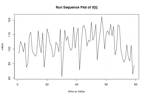
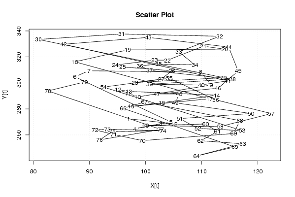
| Dataseries X: | |||||||||||||||||||||||||||||||||||||||||||||||||||||||||||||||||
97 105,4 102,7 98,1 104,5 87,4 89,9 109,8 111,7 98,6 96,9 95,1 97 112,7 102,9 97,4 111,4 87,4 96,8 114,1 110,3 103,9 101,6 94,6 95,9 104,7 102,8 98,1 113,9 80,9 95,7 113,2 105,9 108,8 102,3 99 100,7 115,5 100,7 109,9 114,6 85,4 100,5 114,8 116,5 112,9 102 106 105,3 118,8 106,1 109,3 117,2 92,5 104,2 112,5 122,4 113,3 100 110,7 112,8 109,8 117,3 109,1 115,9 96 99,8 116,8 115,7 99,4 94,3 91 93,2 103,1 94,1 91,8 102,7 82,6 89,1 | |||||||||||||||||||||||||||||||||||||||||||||||||||||||||||||||||
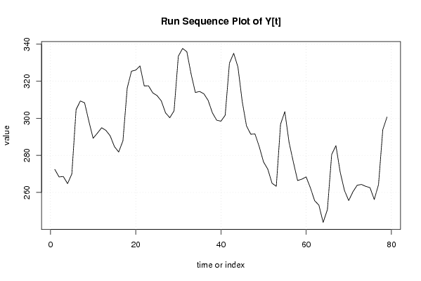
| Dataseries Y: | |||||||||||||||||||||||||||||||||||||||||||||||||||||||||||||||||
272.433 268.361 268.586 264.768 269.974 304.744 309.365 308.347 298.427 289.231 291.975 294.912 293.488 290.555 284.736 281.818 287.854 316.263 325.412 326.011 328.282 317.480 317.539 313.737 312.276 309.391 302.950 300.316 304.035 333.476 337.698 335.932 323.931 313.927 314.485 313.218 309.664 302.963 298.989 298.423 301.631 329.765 335.083 327.616 309.119 295.916 291.413 291.542 284.678 276.475 272.566 264.981 263.290 296.806 303.598 286.994 276.427 266.424 267.153 268.381 262.522 255.542 253.158 243.803 250.741 280.445 285.257 270.976 261.076 255.603 260.376 263.903 264.291 263.276 262.572 256.167 264.221 293.860 300.713 | |||||||||||||||||||||||||||||||||||||||||||||||||||||||||||||||||
Tables (Output of Computation) | |||||||||||||||||||||||||||||||||||||||||||||||||||||||||||||||||
| |||||||||||||||||||||||||||||||||||||||||||||||||||||||||||||||||
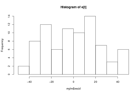
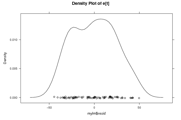
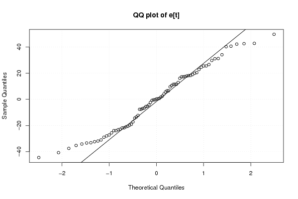
Figures (Output of Computation) | |||||||||||||||||||||||||||||||||||||||||||||||||||||||||||||||||
Input Parameters & R Code | |||||||||||||||||||||||||||||||||||||||||||||||||||||||||||||||||
| Parameters (Session): | |||||||||||||||||||||||||||||||||||||||||||||||||||||||||||||||||
| par1 = 0 ; par2 = 36 ; | |||||||||||||||||||||||||||||||||||||||||||||||||||||||||||||||||
| Parameters (R input): | |||||||||||||||||||||||||||||||||||||||||||||||||||||||||||||||||
| par1 = 0 ; par2 = 36 ; | |||||||||||||||||||||||||||||||||||||||||||||||||||||||||||||||||
| R code (references can be found in the software module): | |||||||||||||||||||||||||||||||||||||||||||||||||||||||||||||||||
par1 <- as.numeric(par1) | |||||||||||||||||||||||||||||||||||||||||||||||||||||||||||||||||