Free Statistics
of Irreproducible Research!
Description of Statistical Computation | |||||||||||||||||||||||||||||||||||||||||||||||||||||||||||||||||
|---|---|---|---|---|---|---|---|---|---|---|---|---|---|---|---|---|---|---|---|---|---|---|---|---|---|---|---|---|---|---|---|---|---|---|---|---|---|---|---|---|---|---|---|---|---|---|---|---|---|---|---|---|---|---|---|---|---|---|---|---|---|---|---|---|---|
| Author's title | |||||||||||||||||||||||||||||||||||||||||||||||||||||||||||||||||
| Author | *The author of this computation has been verified* | ||||||||||||||||||||||||||||||||||||||||||||||||||||||||||||||||
| R Software Module | rwasp_edabi.wasp | ||||||||||||||||||||||||||||||||||||||||||||||||||||||||||||||||
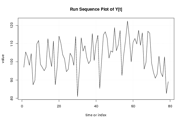
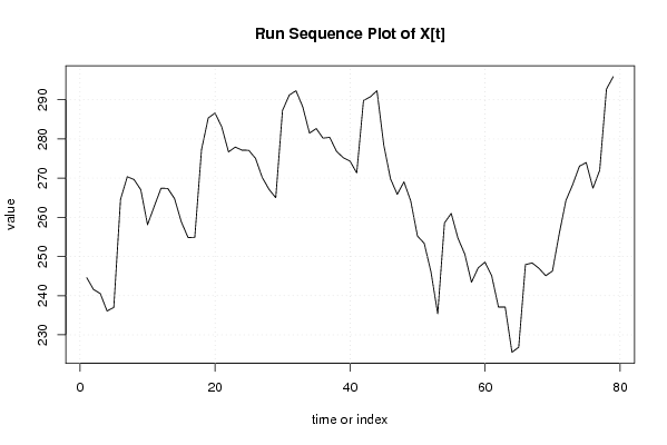
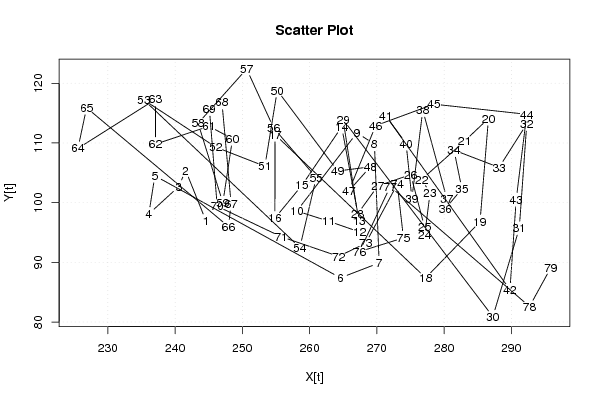
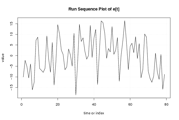
| Title produced by software | Bivariate Explorative Data Analysis | ||||||||||||||||||||||||||||||||||||||||||||||||||||||||||||||||
| Date of computation | Sun, 22 Nov 2009 10:49:18 -0700 | ||||||||||||||||||||||||||||||||||||||||||||||||||||||||||||||||
| Cite this page as follows | Statistical Computations at FreeStatistics.org, Office for Research Development and Education, URL https://freestatistics.org/blog/index.php?v=date/2009/Nov/22/t12589121917wkgegbvvkcuw9l.htm/, Retrieved Sat, 27 Apr 2024 23:57:55 +0000 | ||||||||||||||||||||||||||||||||||||||||||||||||||||||||||||||||
| Statistical Computations at FreeStatistics.org, Office for Research Development and Education, URL https://freestatistics.org/blog/index.php?pk=58671, Retrieved Sat, 27 Apr 2024 23:57:55 +0000 | |||||||||||||||||||||||||||||||||||||||||||||||||||||||||||||||||
| QR Codes: | |||||||||||||||||||||||||||||||||||||||||||||||||||||||||||||||||
|
| |||||||||||||||||||||||||||||||||||||||||||||||||||||||||||||||||
| Original text written by user: | |||||||||||||||||||||||||||||||||||||||||||||||||||||||||||||||||
| IsPrivate? | No (this computation is public) | ||||||||||||||||||||||||||||||||||||||||||||||||||||||||||||||||
| User-defined keywords | |||||||||||||||||||||||||||||||||||||||||||||||||||||||||||||||||
| Estimated Impact | 159 | ||||||||||||||||||||||||||||||||||||||||||||||||||||||||||||||||
Tree of Dependent Computations | |||||||||||||||||||||||||||||||||||||||||||||||||||||||||||||||||
| Family? (F = Feedback message, R = changed R code, M = changed R Module, P = changed Parameters, D = changed Data) | |||||||||||||||||||||||||||||||||||||||||||||||||||||||||||||||||
| - [Bivariate Explorative Data Analysis] [Ws 5 bivariate X ...] [2009-11-04 15:39:55] [62d3ced7fb1c10c35a82e9cb1d0d0e2b] - D [Bivariate Explorative Data Analysis] [Ws 5 bivariate X ...] [2009-11-04 16:22:44] [62d3ced7fb1c10c35a82e9cb1d0d0e2b] - D [Bivariate Explorative Data Analysis] [WS 5 bivariate EDA] [2009-11-22 17:49:18] [b02b8a83db8a631da1ab9c106b4cdcf2] [Current] - D [Bivariate Explorative Data Analysis] [WS 5 Bivariate EDA 1] [2009-11-22 17:53:15] [005293453b571dbccb80b45226e44173] - D [Bivariate Explorative Data Analysis] [WS 5 Bivariate EDA 2] [2009-11-22 18:01:47] [005293453b571dbccb80b45226e44173] | |||||||||||||||||||||||||||||||||||||||||||||||||||||||||||||||||
| Feedback Forum | |||||||||||||||||||||||||||||||||||||||||||||||||||||||||||||||||
Post a new message | |||||||||||||||||||||||||||||||||||||||||||||||||||||||||||||||||
Dataset | |||||||||||||||||||||||||||||||||||||||||||||||||||||||||||||||||
| Dataseries X: | |||||||||||||||||||||||||||||||||||||||||||||||||||||||||||||||||
244.576 241.572 240.541 236.089 236.997 264.579 270.349 269.645 267.037 258.113 262.813 267.413 267.366 264.777 258.863 254.844 254.868 277.267 285.351 286.602 283.042 276.687 277.915 277.128 277.103 275.037 270.150 267.140 264.993 287.259 291.186 292.300 288.186 281.477 282.656 280.190 280.408 276.836 275.216 274.352 271.311 289.802 290.726 292.300 278.506 269.826 265.861 269.034 264.176 255.198 253.353 246.057 235.372 258.556 260.993 254.663 250.643 243.422 247.105 248.541 245.039 237.080 237.085 225.554 226.839 247.934 248.333 246.969 245.098 246.263 255.765 264.319 268.347 273.046 273.963 267.430 271.993 292.710 295.881 | |||||||||||||||||||||||||||||||||||||||||||||||||||||||||||||||||
| Dataseries Y: | |||||||||||||||||||||||||||||||||||||||||||||||||||||||||||||||||
97 105,4 102,7 98,1 104,5 87,4 89,9 109,8 111,7 98,6 96,9 95,1 97 112,7 102,9 97,4 111,4 87,4 96,8 114,1 110,3 103,9 101,6 94,6 95,9 104,7 102,8 98,1 113,9 80,9 95,7 113,2 105,9 108,8 102,3 99 100,7 115,5 100,7 109,9 114,6 85,4 100,5 114,8 116,5 112,9 102 106 105,3 118,8 106,1 109,3 117,2 92,5 104,2 112,5 122,4 113,3 100 110,7 112,8 109,8 117,3 109,1 115,9 96 99,8 116,8 115,7 99,4 94,3 91 93,2 103,1 94,1 91,8 102,7 82,6 89,1 | |||||||||||||||||||||||||||||||||||||||||||||||||||||||||||||||||
Tables (Output of Computation) | |||||||||||||||||||||||||||||||||||||||||||||||||||||||||||||||||
| |||||||||||||||||||||||||||||||||||||||||||||||||||||||||||||||||
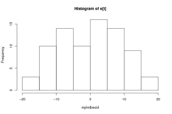
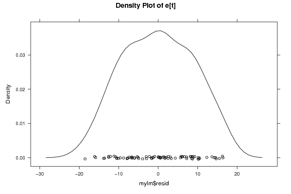
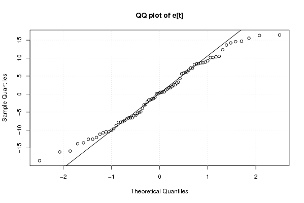
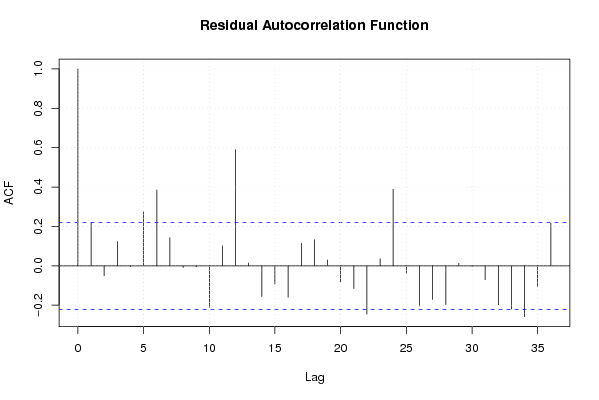
Figures (Output of Computation) | |||||||||||||||||||||||||||||||||||||||||||||||||||||||||||||||||
Input Parameters & R Code | |||||||||||||||||||||||||||||||||||||||||||||||||||||||||||||||||
| Parameters (Session): | |||||||||||||||||||||||||||||||||||||||||||||||||||||||||||||||||
| par1 = 0 ; par2 = 36 ; | |||||||||||||||||||||||||||||||||||||||||||||||||||||||||||||||||
| Parameters (R input): | |||||||||||||||||||||||||||||||||||||||||||||||||||||||||||||||||
| par1 = 0 ; par2 = 36 ; | |||||||||||||||||||||||||||||||||||||||||||||||||||||||||||||||||
| R code (references can be found in the software module): | |||||||||||||||||||||||||||||||||||||||||||||||||||||||||||||||||
par1 <- as.numeric(par1) | |||||||||||||||||||||||||||||||||||||||||||||||||||||||||||||||||