Repository of Reproducible Computations

Free Statistics

of Irreproducible Research!

Author's title

Author

*The author of this computation has been verified*

R Software Module

rwasp_edauni.wasp

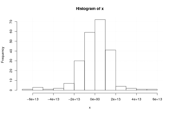
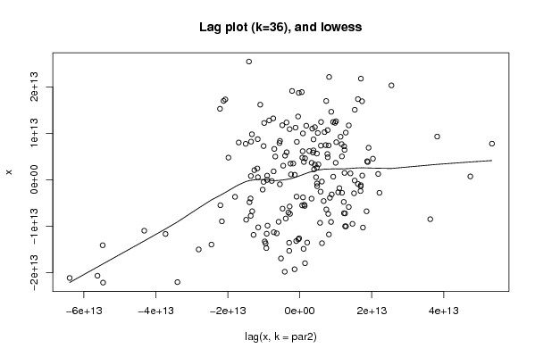
Title produced by software

Univariate Explorative Data Analysis

Date of computation

Sun, 22 Nov 2009 02:17:04 -0700

Cite this page as follows

Statistical Computations at FreeStatistics.org, Office for Research Development and Education, URL https://freestatistics.org/blog/index.php?v=date/2009/Nov/22/t12588815519kxfngfaj9kmcob.htm/, Retrieved Sat, 27 Apr 2024 15:07:24 +0000

Statistical Computations at FreeStatistics.org, Office for Research Development and Education, URL https://freestatistics.org/blog/index.php?pk=58601, Retrieved Sat, 27 Apr 2024 15:07:24 +0000

QR Codes:

Paste this QR Code to cite your computation.

Original text written by user:

IsPrivate?

No (this computation is public)

User-defined keywords

Estimated Impact

178

Family? (F = Feedback message, R = changed R code, M = changed R Module, P = changed Parameters, D = changed Data)

-     [Bivariate Explorative Data Analysis] [SHW_WS4_Q2(2)] [2009-10-23 08:55:58] [8b1aef4e7013bd33fbc2a5833375c5f5]
-  M D  [Bivariate Explorative Data Analysis] [paper] [2009-11-22 08:33:39] [8b1aef4e7013bd33fbc2a5833375c5f5]
- RM D      [Univariate Explorative Data Analysis] [paper] [2009-11-22 09:17:04] [f0f26816ac6124f58333f11f6c174000] [Current]
- R  D        [Univariate Explorative Data Analysis] [model_3et] [2009-12-29 10:04:25] [2663058f2a5dda519058ac6b2228468f] 

Feedback Forum

Post a new message

Dataseries X:

Download CSV

Histogram

Boxplots

-1.02788E+13
-1.18964E+13
-62057298249
7.24304E+12
2.41619E+12
-4.05419E+12
-8.6353E+12
-6.7979E+12
8.19387E+12
1.32084E+13
3.01757E+12
3.47692E+12
1.08919E+13
1.12154E+13
4.60923E+12
3.63868E+12
3.63868E+12
6.41451E+12
5.01673E+12
1.02511E+13
5.53413E+12
7.44932E+12
6.317E+12
2.22116E+12
-6.24218E+12
-5.78283E+12
-8.37098E+12
-7.37449E+12
-3.81579E+12
5.25789E+11
-5.40126E+12
-1.93064E+13
-1.53402E+13
-1.37226E+13
-1.13221E+13
-1.4745E+13
-1.15616E+13
-1.28557E+13
-9.10933E+12
-1.0054E+13
-1.18074E+13
-1.36966E+13
-1.49067E+13
-1.32311E+13
-1.35546E+13
-7.38183E+12
-4.60599E+12
-1.83016E+12
-2.82664E+12
-1.18312E+12
1.45689E+12
3.28809E+12
9.97208E+12
1.24244E+13
1.16996E+13
6.87892E+12
7.66179E+12
7.17651E+12
3.80549E+12
3.96725E+12
-4.79368E+12
-2.82664E+12
-3.9071E+12
-2.72293E+12
8.87629E+11
4.52412E+12
1.23707E+12
-1.45478E+12
-2.93654E+12
-9.51682E+12
-7.22627E+12
-9.30321E+12
-6.41747E+12
-4.06446E+11
8.67801E+12
1.25862E+13
8.08282E+12
6.16764E+12
1.04939E+12
-9.95432E+11
2.05207E+12
7.90133E+12
6.63319E+12
1.10007E+13
2.21362E+13
1.69599E+13
1.24306E+13
5.17735E+12
8.61702E+11
5.90217E+12
1.36148E+13
1.91208E+13
1.1628E+13
1.23269E+13
1.8875E+13
1.87133E+13
1.2217E+13
1.17317E+13
8.36068E+12
1.06772E+13
1.73612E+13
2.03247E+13
2.17805E+13
1.69018E+13
1.50644E+13
1.4631E+13
1.22564E+13
5.62431E+12
7.37773E+12
6.13551E+12
3.81283E+12
1.00634E+13
1.01412E+13
2.61627E+12
-1.39559E+12
-5.54329E+12
-1.26348E+13
-5.65319E+12
-7.0831E+12
3.45719E+12
8.14821E+12
7.33941E+12
9.2546E+12
-4.08745E+12
-9.07606E+12
-3.66022E+12
-4.76891E+11
-2.14634E+12
1.79394E+12
-3.69968E+12
5.31986E+11
-2.7681E+11
-9.90459E+12
-4.86412E+12
-5.51116E+12
7.72718E+12
1.61646E+13
2.54627E+13
1.69734E+13
1.72969E+13
1.5278E+13
8.73606E+12
9.79059E+12
4.75012E+12
8.01124E+12
7.83921E+11
1.13337E+12
4.98966E+12
1.278E+13
4.74393E+12
4.8279E+12
6.48088E+11
-1.86636E+11
1.35318E+12
-3.17609E+12
-2.5809E+12
-8.27476E+11
5.85651E+12
1.13242E+13
3.25597E+12
-5.88653E+12
-8.97921E+11
-1.0054E+13
-1.03194E+13
-7.27192E+12
-1.80061E+13
-1.16456E+13
-7.78933E+12
-8.9735E+12
-1.3988E+13
-2.2076E+13
-1.50426E+13
-1.09986E+13
-1.41301E+13
-2.11894E+13
-2.07041E+13
-2.21859E+13
-1.16975E+13
-1.33151E+13
-1.98373E+13
-1.69775E+13
-1.36065E+13
-2.44507E+12
-6.81257E+12
-8.51414E+12
6.99943E+11
7.7593E+12
9.29292E+12
1.52521E+13
1.40679E+13
8.86569E+12
5.76634E+12
4.76985E+12
3.66347E+12
4.2006E+12
4.17467E+12
1.36086E+13
1.61387E+13
1.28257E+13
1.75426E+13
1.258E+13
1.44449E+12
-9.2057E+12
-1.3651E+13
-2.1655E+13
-2.45666E+13
-3.40067E+13
-2.81056E+13
-4.32332E+13
-5.47959E+13
-6.39779E+13
-5.62394E+13
-5.46798E+13
-3.73259E+13
-9.74903E+12
-4.19116E+12
-5.2333E+12
-2.96247E+12
1.68821E+13
1.85515E+13
3.62611E+13
4.73965E+13
5.34138E+13
3.81825E+13

Summary of computational transaction
Raw Input	view raw input (R code)
Raw Output	view raw output of R engine
Computing time	3 seconds
R Server	'Gwilym Jenkins' @ 72.249.127.135

\begin{tabular}{lllllllll}
\hline
Summary of computational transaction \tabularnewline
Raw Input & view raw input (R code)  \tabularnewline
Raw Output & view raw output of R engine  \tabularnewline
Computing time & 3 seconds \tabularnewline
R Server & 'Gwilym Jenkins' @ 72.249.127.135 \tabularnewline
\hline
\end{tabular}
%Source: https://freestatistics.org/blog/index.php?pk=58601&T=0

[TABLE]
[ROW][C]Summary of computational transaction[/C][/ROW]
[ROW][C]Raw Input[/C][C]view raw input (R code) [/C][/ROW]
[ROW][C]Raw Output[/C][C]view raw output of R engine [/C][/ROW]
[ROW][C]Computing time[/C][C]3 seconds[/C][/ROW]
[ROW][C]R Server[/C][C]'Gwilym Jenkins' @ 72.249.127.135[/C][/ROW]
[/TABLE]
Source: https://freestatistics.org/blog/index.php?pk=58601&T=0

Globally Unique Identifier (entire table): ba.freestatistics.org/blog/index.php?pk=58601&T=0

As an alternative you can also use a QR Code:

The GUIDs for individual cells are displayed in the table below:

Summary of computational transaction
Raw Input	view raw input (R code)
Raw Output	view raw output of R engine
Computing time	3 seconds
R Server	'Gwilym Jenkins' @ 72.249.127.135

Descriptive Statistics
# observations	224
minimum	-6.39779e+13
Q1	-7.483705e+12
median	1.18522e+12
mean	1288847.10267765
Q3	8440012500000
maximum	5.34138e+13

\begin{tabular}{lllllllll}
\hline
Descriptive Statistics \tabularnewline
# observations & 224 \tabularnewline
minimum & -6.39779e+13 \tabularnewline
Q1 & -7.483705e+12 \tabularnewline
median & 1.18522e+12 \tabularnewline
mean & 1288847.10267765 \tabularnewline
Q3 & 8440012500000 \tabularnewline
maximum & 5.34138e+13 \tabularnewline
\hline
\end{tabular}
%Source: https://freestatistics.org/blog/index.php?pk=58601&T=1

[TABLE]
[ROW][C]Descriptive Statistics[/C][/ROW]
[ROW][C]# observations[/C][C]224[/C][/ROW]
[ROW][C]minimum[/C][C]-6.39779e+13[/C][/ROW]
[ROW][C]Q1[/C][C]-7.483705e+12[/C][/ROW]
[ROW][C]median[/C][C]1.18522e+12[/C][/ROW]
[ROW][C]mean[/C][C]1288847.10267765[/C][/ROW]
[ROW][C]Q3[/C][C]8440012500000[/C][/ROW]
[ROW][C]maximum[/C][C]5.34138e+13[/C][/ROW]
[/TABLE]
Source: https://freestatistics.org/blog/index.php?pk=58601&T=1

Globally Unique Identifier (entire table): ba.freestatistics.org/blog/index.php?pk=58601&T=1

As an alternative you can also use a QR Code:

The GUIDs for individual cells are displayed in the table below:

Descriptive Statistics
# observations	224
minimum	-6.39779e+13
Q1	-7.483705e+12
median	1.18522e+12
mean	1288847.10267765
Q3	8440012500000
maximum	5.34138e+13

Figure 1

PNG link

Postscript link

PDF link

Figure 2

PNG link

Postscript link

PDF link

Figure 3

PNG link

Postscript link

PDF link

Figure 4

PNG link

Postscript link

PDF link

Figure 5

PNG link

Postscript link

PDF link

Figure 6

PNG link

Postscript link

PDF link

Figure 7

PNG link

Postscript link

PDF link

Parameters (Session):

par1 = 0 ; par2 = 36 ;

Parameters (R input):

par1 = 0 ; par2 = 36 ;

R code (references can be found in the software module):

par1 <- as.numeric(par1)
par2 <- as.numeric(par2)
x <- as.ts(x)
library(lattice)
bitmap(file='pic1.png')
plot(x,type='l',main='Run Sequence Plot',xlab='time or index',ylab='value')
grid()
dev.off()
bitmap(file='pic2.png')
hist(x)
grid()
dev.off()
bitmap(file='pic3.png')
if (par1 > 0)
{
densityplot(~x,col='black',main=paste('Density Plot   bw = ',par1),bw=par1)
} else {
densityplot(~x,col='black',main='Density Plot')
}
dev.off()
bitmap(file='pic4.png')
qqnorm(x)
qqline(x)
grid()
dev.off()
if (par2 > 0)
{
bitmap(file='lagplot1.png')
dum <- cbind(lag(x,k=1),x)
dum
dum1 <- dum[2:length(x),]
dum1
z <- as.data.frame(dum1)
z
plot(z,main='Lag plot (k=1), lowess, and regression line')
lines(lowess(z))
abline(lm(z))
dev.off()
if (par2 > 1) {
bitmap(file='lagplotpar2.png')
dum <- cbind(lag(x,k=par2),x)
dum
dum1 <- dum[(par2+1):length(x),]
dum1
z <- as.data.frame(dum1)
z
mylagtitle <- 'Lag plot (k='
mylagtitle <- paste(mylagtitle,par2,sep='')
mylagtitle <- paste(mylagtitle,'), and lowess',sep='')
plot(z,main=mylagtitle)
lines(lowess(z))
dev.off()
}
bitmap(file='pic5.png')
acf(x,lag.max=par2,main='Autocorrelation Function')
grid()
dev.off()
}
summary(x)
load(file='createtable')
a<-table.start()
a<-table.row.start(a)
a<-table.element(a,'Descriptive Statistics',2,TRUE)
a<-table.row.end(a)
a<-table.row.start(a)
a<-table.element(a,'# observations',header=TRUE)
a<-table.element(a,length(x))
a<-table.row.end(a)
a<-table.row.start(a)
a<-table.element(a,'minimum',header=TRUE)
a<-table.element(a,min(x))
a<-table.row.end(a)
a<-table.row.start(a)
a<-table.element(a,'Q1',header=TRUE)
a<-table.element(a,quantile(x,0.25))
a<-table.row.end(a)
a<-table.row.start(a)
a<-table.element(a,'median',header=TRUE)
a<-table.element(a,median(x))
a<-table.row.end(a)
a<-table.row.start(a)
a<-table.element(a,'mean',header=TRUE)
a<-table.element(a,mean(x))
a<-table.row.end(a)
a<-table.row.start(a)
a<-table.element(a,'Q3',header=TRUE)
a<-table.element(a,quantile(x,0.75))
a<-table.row.end(a)
a<-table.row.start(a)
a<-table.element(a,'maximum',header=TRUE)
a<-table.element(a,max(x))
a<-table.row.end(a)
a<-table.end(a)
table.save(a,file='mytable.tab')

Free Statistics

Description of Statistical Computation

Tree of Dependent Computations

Dataset

Tables (Output of Computation)

Figures (Output of Computation)

Input Parameters & R Code