Free Statistics
of Irreproducible Research!
Description of Statistical Computation | |||||||||||||||||||||||||||||||||||||||||||||||||||||||||||||||||
|---|---|---|---|---|---|---|---|---|---|---|---|---|---|---|---|---|---|---|---|---|---|---|---|---|---|---|---|---|---|---|---|---|---|---|---|---|---|---|---|---|---|---|---|---|---|---|---|---|---|---|---|---|---|---|---|---|---|---|---|---|---|---|---|---|---|
| Author's title | |||||||||||||||||||||||||||||||||||||||||||||||||||||||||||||||||
| Author | *The author of this computation has been verified* | ||||||||||||||||||||||||||||||||||||||||||||||||||||||||||||||||
| R Software Module | rwasp_edabi.wasp | ||||||||||||||||||||||||||||||||||||||||||||||||||||||||||||||||
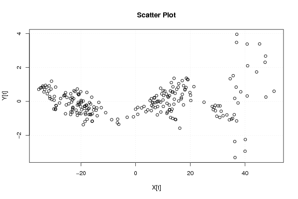
| Title produced by software | Bivariate Explorative Data Analysis | ||||||||||||||||||||||||||||||||||||||||||||||||||||||||||||||||
| Date of computation | Sun, 22 Nov 2009 01:33:39 -0700 | ||||||||||||||||||||||||||||||||||||||||||||||||||||||||||||||||
| Cite this page as follows | Statistical Computations at FreeStatistics.org, Office for Research Development and Education, URL https://freestatistics.org/blog/index.php?v=date/2009/Nov/22/t12588789210q2be4xp68eyvft.htm/, Retrieved Sat, 27 Apr 2024 18:20:41 +0000 | ||||||||||||||||||||||||||||||||||||||||||||||||||||||||||||||||
| Statistical Computations at FreeStatistics.org, Office for Research Development and Education, URL https://freestatistics.org/blog/index.php?pk=58600, Retrieved Sat, 27 Apr 2024 18:20:41 +0000 | |||||||||||||||||||||||||||||||||||||||||||||||||||||||||||||||||
| QR Codes: | |||||||||||||||||||||||||||||||||||||||||||||||||||||||||||||||||
|
| |||||||||||||||||||||||||||||||||||||||||||||||||||||||||||||||||
| Original text written by user: | |||||||||||||||||||||||||||||||||||||||||||||||||||||||||||||||||
| IsPrivate? | No (this computation is public) | ||||||||||||||||||||||||||||||||||||||||||||||||||||||||||||||||
| User-defined keywords | |||||||||||||||||||||||||||||||||||||||||||||||||||||||||||||||||
| Estimated Impact | 162 | ||||||||||||||||||||||||||||||||||||||||||||||||||||||||||||||||
Tree of Dependent Computations | |||||||||||||||||||||||||||||||||||||||||||||||||||||||||||||||||
| Family? (F = Feedback message, R = changed R code, M = changed R Module, P = changed Parameters, D = changed Data) | |||||||||||||||||||||||||||||||||||||||||||||||||||||||||||||||||
| - [Bivariate Explorative Data Analysis] [SHW_WS4_Q2(2)] [2009-10-23 08:55:58] [8b1aef4e7013bd33fbc2a5833375c5f5] - M D [Bivariate Explorative Data Analysis] [paper] [2009-11-22 08:33:39] [f0f26816ac6124f58333f11f6c174000] [Current] - RM D [Univariate Explorative Data Analysis] [paper] [2009-11-22 09:17:04] [8b1aef4e7013bd33fbc2a5833375c5f5] - R D [Univariate Explorative Data Analysis] [model_3et] [2009-12-29 10:04:25] [2663058f2a5dda519058ac6b2228468f] | |||||||||||||||||||||||||||||||||||||||||||||||||||||||||||||||||
| Feedback Forum | |||||||||||||||||||||||||||||||||||||||||||||||||||||||||||||||||
Post a new message | |||||||||||||||||||||||||||||||||||||||||||||||||||||||||||||||||
Dataset | |||||||||||||||||||||||||||||||||||||||||||||||||||||||||||||||||
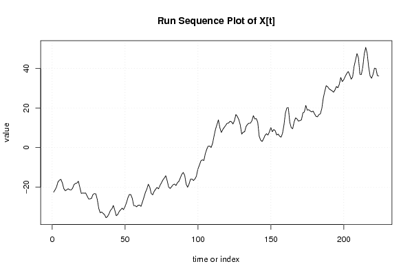
| Dataseries X: | |||||||||||||||||||||||||||||||||||||||||||||||||||||||||||||||||
-22.55812594 -21.35812594 -19.86358022 -17.3690345 -16.47448878 -16.07448878 -17.86358022 -20.74176309 -21.83085453 -21.33085453 -20.83085453 -21.32540024 -21.41994596 -20.61994596 -18.72540024 -18.12540024 -17.92540024 -17.03085453 -20.1090374 -23.18722027 -22.98176599 -23.0763117 -22.9763117 -24.46540314 -25.95449458 -25.94904029 -25.64904029 -23.75449458 -23.25449458 -23.44904029 -26.32722316 -30.79449747 -32.97813462 -32.57813462 -33.27268034 -33.96722606 -35.4563175 -34.8563175 -33.56177178 -31.76722606 -30.97268034 -29.28358891 -31.66722606 -34.44540893 -33.84540893 -32.35086321 -31.4563175 -30.66177178 -31.3563175 -29.86177178 -27.87268034 -25.38358891 -23.69449747 -23.79995175 -25.68358891 -29.3563175 -29.35086321 -29.95086321 -29.1563175 -29.0563175 -29.75086321 -27.4563175 -25.16722606 -22.67813462 -20.98904319 -18.50540604 -19.99449747 -23.17268034 -23.86722606 -22.17813462 -21.08358891 -20.08904319 -20.88358891 -19.18904319 -17.79449747 -16.39995175 -15.40540604 -14.21086032 -16.88904319 -19.96722606 -20.66177178 -19.76722606 -18.77268034 -18.47268034 -19.16722606 -17.76722606 -17.06722606 -15.27268034 -13.48358891 -12.58904319 -14.07813462 -18.54540893 -20.03450037 -18.34540893 -15.96177178 -15.86177178 -16.6563175 -15.8563175 -14.46177178 -10.97268034 -8.783588907 -6.694497471 -6.194497471 -6.589043189 -3.110860318 -0.821768882 0.767322553 0.767322553 -0.027223164 2.161868271 5.840051143 9.218234014 11.60187117 13.98550832 10.01277973 7.63459686 9.129142578 10.2236883 11.21823401 12.31277973 12.41277973 13.31277973 13.01823401 11.93459686 13.62914258 16.71277973 15.7236883 14.13459686 11.45641399 6.789139682 7.7836854 7.9836854 10.66732255 11.76186827 12.36186827 12.36732255 13.56186827 16.14550542 14.46186827 14.66186827 12.77823112 5.727319657 3.743682504 3.049136786 4.443682504 6.132773939 7.027319657 6.332773939 7.927319657 10.11641109 8.032773939 9.127319657 8.532773939 6.349136786 6.849136786 5.76004535 5.265499632 7.154591068 11.42731966 17.48913968 20.07277684 20.17823112 12.73277394 10.05459107 9.56004535 13.03822822 15.02731966 14.43277394 13.3436825 13.6436825 14.0436825 17.52731966 18.02731966 21.30550253 18.92731966 19.12731966 18.53277394 18.03822822 18.43822822 17.04913679 15.76004535 15.56549963 16.66549963 17.06549963 19.84913679 25.01641109 28.39459396 31.27823112 30.7836854 29.69459396 29.20004825 28.70550253 28.01095681 29.10550253 30.89459396 30.20004825 31.98913968 35.46732255 33.3836854 34.27823112 36.06732255 37.46186827 38.45641399 36.77277684 34.58913968 35.68913968 40.96732255 44.25095971 47.53459686 45.35095971 37.01095681 36.91641109 40.79459396 47.35095971 50.63459686 47.65641399 40.80550253 36.23822822 35.04913679 36.93822822 40.12186538 40.02731966 36.35459107 36.26004535 | |||||||||||||||||||||||||||||||||||||||||||||||||||||||||||||||||
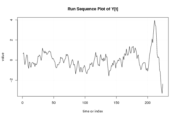
| Dataseries Y: | |||||||||||||||||||||||||||||||||||||||||||||||||||||||||||||||||
0.635439214 0.735439214 0.003836396 -0.447766422 -0.14936924 0.25063076 0.533836396 0.420247668 -0.506546695 -0.816546695 -0.186546695 -0.214943877 -0.673341059 -0.693341059 -0.284943877 -0.224943877 -0.224943877 -0.396546695 -0.310135423 -0.63372415 -0.342121332 -0.460518514 -0.390518514 -0.137312877 0.385892759 0.357495577 0.517495577 0.455892759 0.235892759 -0.032504423 0.33390685 1.193523758 0.948332213 0.848332213 0.699935031 0.911537849 0.714743485 0.794743485 0.563140667 0.621537849 0.729935031 0.846729395 0.921537849 0.817949122 0.837949122 0.456346304 0.284743485 0.113140667 0.174743485 0.073140667 -0.090064969 -0.203270605 -0.616476242 -0.76807906 -0.723270605 -0.425256515 -0.473653696 -0.443653696 -0.235256515 -0.245256515 0.296346304 0.174743485 0.241537849 0.168332213 -0.054873423 -0.279681878 -0.076476242 0.089935031 0.181537849 0.588332213 0.446729395 0.575126577 0.396729395 0.025126577 -0.536476242 -0.77807906 -0.499681878 -0.381284696 -0.064873423 0.061537849 -0.126859333 -0.488462151 -0.410064969 -0.680064969 -1.368462151 -1.048462151 -0.768462151 -0.320064969 -0.053270605 -0.364873423 -0.841667787 -1.182050878 -0.718845242 -0.762050878 -1.166859333 -1.156859333 -0.755256515 -0.725256515 -0.516859333 -0.660064969 -1.073270605 -1.256476242 -1.346476242 -1.044873423 -0.931284696 -0.904490332 -0.757695969 -0.347695969 -0.45609315 -0.379298787 -0.235710059 -0.622121332 -0.626929786 -0.161738241 0.08627585 0.342687123 0.781084304 0.349481486 0.437878668 -0.21372415 -0.50372415 -0.45372415 -0.572121332 0.252687123 0.561084304 0.22627585 0.029481486 0.132687123 -0.110901605 0.228715304 -0.032887514 0.017112486 0.612304031 0.300701213 0.340701213 -0.477695969 -0.999298787 -1.574107241 -1.049298787 -1.069298787 -0.944490332 -0.540064969 -0.605256515 -0.293653696 -0.495256515 -0.048462151 -0.070064969 -0.308462151 -0.790064969 -0.293270605 -0.298462151 -0.040064969 0.011537849 -0.083653696 0.196346304 0.15955194 0.051154758 -0.362050878 -0.700064969 -0.201284696 0.36390685 0.055509668 0.621537849 0.637949122 0.44955194 1.113140667 0.719935031 0.481537849 0.554743485 0.864743485 1.364743485 0.929935031 0.679935031 0.873523758 1.309935031 1.279935031 1.371537849 0.723140667 0.823140667 1.226346304 1.04955194 0.841154758 0.151154758 0.421154758 0.526346304 -0.043270605 -0.479681878 -0.574490332 -0.942887514 -0.869681878 -0.54807906 -0.356476242 -0.294873423 -0.226476242 -0.259681878 -0.25807906 -0.841284696 -0.997695969 -0.792887514 -1.084490332 -0.777695969 -0.089298787 0.569098395 0.84390685 1.338715304 1.518715304 2.102304031 1.737495577 2.672687123 3.387495577 3.955126577 3.476729395 3.380318122 2.307495577 0.602687123 0.259098395 0.323523758 0.183140667 -1.043653696 -1.146859333 -2.241667787 -2.930064969 -3.302050878 -2.36044806 | |||||||||||||||||||||||||||||||||||||||||||||||||||||||||||||||||
Tables (Output of Computation) | |||||||||||||||||||||||||||||||||||||||||||||||||||||||||||||||||
| |||||||||||||||||||||||||||||||||||||||||||||||||||||||||||||||||
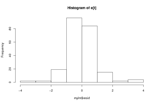
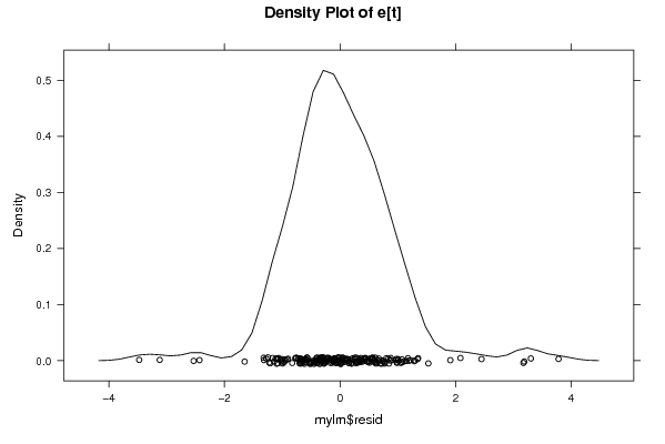
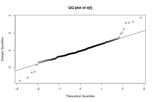
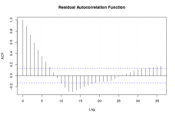
Figures (Output of Computation) | |||||||||||||||||||||||||||||||||||||||||||||||||||||||||||||||||
Input Parameters & R Code | |||||||||||||||||||||||||||||||||||||||||||||||||||||||||||||||||
| Parameters (Session): | |||||||||||||||||||||||||||||||||||||||||||||||||||||||||||||||||
| par1 = 0 ; par2 = 36 ; | |||||||||||||||||||||||||||||||||||||||||||||||||||||||||||||||||
| Parameters (R input): | |||||||||||||||||||||||||||||||||||||||||||||||||||||||||||||||||
| par1 = 0 ; par2 = 36 ; | |||||||||||||||||||||||||||||||||||||||||||||||||||||||||||||||||
| R code (references can be found in the software module): | |||||||||||||||||||||||||||||||||||||||||||||||||||||||||||||||||
par1 <- as.numeric(par1) | |||||||||||||||||||||||||||||||||||||||||||||||||||||||||||||||||