Free Statistics
of Irreproducible Research!
Description of Statistical Computation | |||||||||||||||||||||||||||||||||||||||||||||
|---|---|---|---|---|---|---|---|---|---|---|---|---|---|---|---|---|---|---|---|---|---|---|---|---|---|---|---|---|---|---|---|---|---|---|---|---|---|---|---|---|---|---|---|---|---|
| Author's title | |||||||||||||||||||||||||||||||||||||||||||||
| Author | *The author of this computation has been verified* | ||||||||||||||||||||||||||||||||||||||||||||
| R Software Module | rwasp_boxcoxlin.wasp | ||||||||||||||||||||||||||||||||||||||||||||
| Title produced by software | Box-Cox Linearity Plot | ||||||||||||||||||||||||||||||||||||||||||||
| Date of computation | Fri, 20 Nov 2009 07:18:23 -0700 | ||||||||||||||||||||||||||||||||||||||||||||
| Cite this page as follows | Statistical Computations at FreeStatistics.org, Office for Research Development and Education, URL https://freestatistics.org/blog/index.php?v=date/2009/Nov/20/t1258726784w63jcl9r3qwqseg.htm/, Retrieved Sat, 20 Apr 2024 10:22:33 +0000 | ||||||||||||||||||||||||||||||||||||||||||||
| Statistical Computations at FreeStatistics.org, Office for Research Development and Education, URL https://freestatistics.org/blog/index.php?pk=58195, Retrieved Sat, 20 Apr 2024 10:22:33 +0000 | |||||||||||||||||||||||||||||||||||||||||||||
| QR Codes: | |||||||||||||||||||||||||||||||||||||||||||||
|
| |||||||||||||||||||||||||||||||||||||||||||||
| Original text written by user: | |||||||||||||||||||||||||||||||||||||||||||||
| IsPrivate? | No (this computation is public) | ||||||||||||||||||||||||||||||||||||||||||||
| User-defined keywords | |||||||||||||||||||||||||||||||||||||||||||||
| Estimated Impact | 117 | ||||||||||||||||||||||||||||||||||||||||||||
Tree of Dependent Computations | |||||||||||||||||||||||||||||||||||||||||||||
| Family? (F = Feedback message, R = changed R code, M = changed R Module, P = changed Parameters, D = changed Data) | |||||||||||||||||||||||||||||||||||||||||||||
| - [Back to Back Histogram] [Back2Back] [2009-11-08 13:48:34] [f15cf5036ae52d4243ad71d4fb151dbe] - RMPD [Box-Cox Linearity Plot] [Workshop6/Box cox] [2009-11-20 14:18:23] [f94f05f163a3ee3ab544c4fef41db0eb] [Current] | |||||||||||||||||||||||||||||||||||||||||||||
| Feedback Forum | |||||||||||||||||||||||||||||||||||||||||||||
Post a new message | |||||||||||||||||||||||||||||||||||||||||||||
Dataset | |||||||||||||||||||||||||||||||||||||||||||||
| Dataseries X: | |||||||||||||||||||||||||||||||||||||||||||||
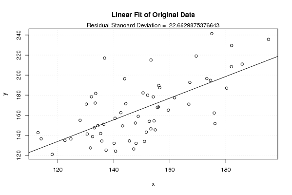
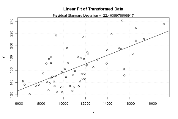
114,08 112,95 135,31 134,31 133,03 140,11 124,69 131,68 150,95 137,26 130,51 143,15 118,01 122,56 147,97 135,74 151,62 154,82 145,59 147,12 175,86 140,66 152,69 154,38 132,45 136,44 153,24 154,11 155,93 142,53 148,73 147,73 166,79 144,30 156,07 161,70 152,10 140,45 155,56 174,53 167,16 159,48 173,22 176,13 180,31 185,84 169,43 195,25 174,99 156,42 182,08 182,00 153,28 136,72 130,19 132,04 143,89 133,38 127,98 150,45 133,55 | |||||||||||||||||||||||||||||||||||||||||||||
| Dataseries Y: | |||||||||||||||||||||||||||||||||||||||||||||
136,49 142,62 141,71 149,51 147,39 131,96 136,38 127,34 133,85 125,14 141,25 149,32 120,92 134,85 131,93 134,22 143,07 145,37 134,32 126,31 162,21 124,09 153,91 154,34 138,70 150,98 146,39 178,30 168,23 162,52 158,86 152,17 171,01 171,49 189,62 177,46 179,98 156,96 167,89 194,78 192,78 165,06 196,60 151,64 187,02 210,99 219,08 235,68 241,44 187,46 229,57 208,44 215,09 217,00 171,08 178,41 196,34 172,11 154,93 182,26 181,74 | |||||||||||||||||||||||||||||||||||||||||||||
Tables (Output of Computation) | |||||||||||||||||||||||||||||||||||||||||||||
| |||||||||||||||||||||||||||||||||||||||||||||
Figures (Output of Computation) | |||||||||||||||||||||||||||||||||||||||||||||
Input Parameters & R Code | |||||||||||||||||||||||||||||||||||||||||||||
| Parameters (Session): | |||||||||||||||||||||||||||||||||||||||||||||
| Parameters (R input): | |||||||||||||||||||||||||||||||||||||||||||||
| R code (references can be found in the software module): | |||||||||||||||||||||||||||||||||||||||||||||
n <- length(x) | |||||||||||||||||||||||||||||||||||||||||||||