Free Statistics
of Irreproducible Research!
Description of Statistical Computation | |||||||||||||||||||||
|---|---|---|---|---|---|---|---|---|---|---|---|---|---|---|---|---|---|---|---|---|---|
| Author's title | |||||||||||||||||||||
| Author | *The author of this computation has been verified* | ||||||||||||||||||||
| R Software Module | rwasp_meanplot.wasp | ||||||||||||||||||||
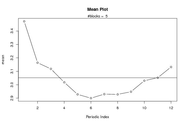
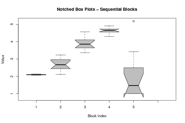
| Title produced by software | Mean Plot | ||||||||||||||||||||
| Date of computation | Fri, 13 Nov 2009 15:39:30 -0700 | ||||||||||||||||||||
| Cite this page as follows | Statistical Computations at FreeStatistics.org, Office for Research Development and Education, URL https://freestatistics.org/blog/index.php?v=date/2009/Nov/13/t1258152021qs0vuh3qkvq21rr.htm/, Retrieved Sun, 05 May 2024 17:23:03 +0000 | ||||||||||||||||||||
| Statistical Computations at FreeStatistics.org, Office for Research Development and Education, URL https://freestatistics.org/blog/index.php?pk=57172, Retrieved Sun, 05 May 2024 17:23:03 +0000 | |||||||||||||||||||||
| QR Codes: | |||||||||||||||||||||
|
| |||||||||||||||||||||
| Original text written by user: | |||||||||||||||||||||
| IsPrivate? | No (this computation is public) | ||||||||||||||||||||
| User-defined keywords | |||||||||||||||||||||
| Estimated Impact | 127 | ||||||||||||||||||||
Tree of Dependent Computations | |||||||||||||||||||||
| Family? (F = Feedback message, R = changed R code, M = changed R Module, P = changed Parameters, D = changed Data) | |||||||||||||||||||||
| - [Partial Correlation] [WS5 (Y[t] - g - h...] [2009-11-04 16:27:45] [8733f8ed033058987ec00f5e71b74854] - D [Partial Correlation] [WS6 Multivariate EDA] [2009-11-13 21:31:18] [8733f8ed033058987ec00f5e71b74854] - RM D [Bagplot] [WS6 Multivariate EDA] [2009-11-13 22:07:10] [8733f8ed033058987ec00f5e71b74854] - RM D [Bivariate Explorative Data Analysis] [WS6 Multivariate EDA] [2009-11-13 22:26:03] [8733f8ed033058987ec00f5e71b74854] - RM D [Mean Plot] [WS6 Multivariate EDA] [2009-11-13 22:39:30] [c6e373ff11c42d4585d53e9e88ed5606] [Current] | |||||||||||||||||||||
| Feedback Forum | |||||||||||||||||||||
Post a new message | |||||||||||||||||||||
Dataset | |||||||||||||||||||||
| Dataseries X: | |||||||||||||||||||||
2,08 2,12 2,14 2,13 2,1 2,09 2,1 2,09 2,08 2,07 2,08 2,09 2,11 2,2 2,42 2,46 2,5 2,59 2,75 2,78 2,9 3,03 3,1 3,23 3,36 3,51 3,61 3,67 3,74 3,82 3,89 3,98 4,08 4,14 4,33 4,57 4,63 4,57 4,71 4,54 4,3 4,36 4,61 4,71 4,68 4,91 4,75 4,77 5,18 3,42 2,71 2,29 2 1,64 1,3 1,08 1 1 1 1 | |||||||||||||||||||||
Tables (Output of Computation) | |||||||||||||||||||||
| |||||||||||||||||||||
Figures (Output of Computation) | |||||||||||||||||||||
Input Parameters & R Code | |||||||||||||||||||||
| Parameters (Session): | |||||||||||||||||||||
| Parameters (R input): | |||||||||||||||||||||
| par1 = 12 ; | |||||||||||||||||||||
| R code (references can be found in the software module): | |||||||||||||||||||||
par1 <- as.numeric(par1) | |||||||||||||||||||||