Free Statistics
of Irreproducible Research!
Description of Statistical Computation | |||||||||||||||||||||
|---|---|---|---|---|---|---|---|---|---|---|---|---|---|---|---|---|---|---|---|---|---|
| Author's title | |||||||||||||||||||||
| Author | *The author of this computation has been verified* | ||||||||||||||||||||
| R Software Module | rwasp_meanplot.wasp | ||||||||||||||||||||
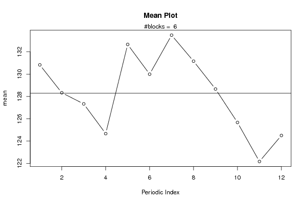
| Title produced by software | Mean Plot | ||||||||||||||||||||
| Date of computation | Fri, 13 Nov 2009 08:00:21 -0700 | ||||||||||||||||||||
| Cite this page as follows | Statistical Computations at FreeStatistics.org, Office for Research Development and Education, URL https://freestatistics.org/blog/index.php?v=date/2009/Nov/13/t1258124474wx7rsgoxnj6b06v.htm/, Retrieved Sun, 05 May 2024 11:59:54 +0000 | ||||||||||||||||||||
| Statistical Computations at FreeStatistics.org, Office for Research Development and Education, URL https://freestatistics.org/blog/index.php?pk=56767, Retrieved Sun, 05 May 2024 11:59:54 +0000 | |||||||||||||||||||||
| QR Codes: | |||||||||||||||||||||
|
| |||||||||||||||||||||
| Original text written by user: | |||||||||||||||||||||
| IsPrivate? | No (this computation is public) | ||||||||||||||||||||
| User-defined keywords | |||||||||||||||||||||
| Estimated Impact | 127 | ||||||||||||||||||||
Tree of Dependent Computations | |||||||||||||||||||||
| Family? (F = Feedback message, R = changed R code, M = changed R Module, P = changed Parameters, D = changed Data) | |||||||||||||||||||||
| - [Kendall tau Correlation Matrix] [3/11/2009] [2009-11-02 21:25:00] [b98453cac15ba1066b407e146608df68] - RMPD [Mean Plot] [] [2009-11-13 15:00:21] [14869f38c4320b00c96ca15cc00142de] [Current] | |||||||||||||||||||||
| Feedback Forum | |||||||||||||||||||||
Post a new message | |||||||||||||||||||||
Dataset | |||||||||||||||||||||
| Dataseries X: | |||||||||||||||||||||
152 148 148 157 157 162 174 158 166 161 147 160 157 147 144 151 154 143 144 137 127 122 124 121 122 112 114 109 117 123 126 127 117 109 105 107 106 111 106 79 112 103 106 123 118 125 122 126 126 132 134 135 135 133 133 127 129 123 121 122 122 120 118 117 121 116 118 115 115 114 114 111 | |||||||||||||||||||||
Tables (Output of Computation) | |||||||||||||||||||||
| |||||||||||||||||||||
Figures (Output of Computation) | |||||||||||||||||||||
Input Parameters & R Code | |||||||||||||||||||||
| Parameters (Session): | |||||||||||||||||||||
| par1 = 12 ; | |||||||||||||||||||||
| Parameters (R input): | |||||||||||||||||||||
| par1 = 12 ; | |||||||||||||||||||||
| R code (references can be found in the software module): | |||||||||||||||||||||
par1 <- as.numeric(par1) | |||||||||||||||||||||