Free Statistics
of Irreproducible Research!
Description of Statistical Computation | |||||||||||||||||||||
|---|---|---|---|---|---|---|---|---|---|---|---|---|---|---|---|---|---|---|---|---|---|
| Author's title | |||||||||||||||||||||
| Author | *The author of this computation has been verified* | ||||||||||||||||||||
| R Software Module | rwasp_sdplot.wasp | ||||||||||||||||||||
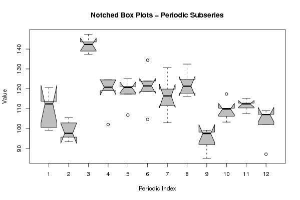
| Title produced by software | Standard Deviation Plot | ||||||||||||||||||||
| Date of computation | Fri, 13 Nov 2009 07:08:04 -0700 | ||||||||||||||||||||
| Cite this page as follows | Statistical Computations at FreeStatistics.org, Office for Research Development and Education, URL https://freestatistics.org/blog/index.php?v=date/2009/Nov/13/t1258121352i2z4jlppa40jqjr.htm/, Retrieved Sun, 05 May 2024 16:45:36 +0000 | ||||||||||||||||||||
| Statistical Computations at FreeStatistics.org, Office for Research Development and Education, URL https://freestatistics.org/blog/index.php?pk=56650, Retrieved Sun, 05 May 2024 16:45:36 +0000 | |||||||||||||||||||||
| QR Codes: | |||||||||||||||||||||
|
| |||||||||||||||||||||
| Original text written by user: | |||||||||||||||||||||
| IsPrivate? | No (this computation is public) | ||||||||||||||||||||
| User-defined keywords | Workshop 6 - Standard Deviation Plot | ||||||||||||||||||||
| Estimated Impact | 158 | ||||||||||||||||||||
Tree of Dependent Computations | |||||||||||||||||||||
| Family? (F = Feedback message, R = changed R code, M = changed R Module, P = changed Parameters, D = changed Data) | |||||||||||||||||||||
| - [Bivariate Data Series] [Bivariate dataset] [2008-01-05 23:51:08] [74be16979710d4c4e7c6647856088456] - RMPD [Bivariate Explorative Data Analysis] [Ws4 part 1.1 s090...] [2009-10-27 21:56:53] [e0fc65a5811681d807296d590d5b45de] - D [Bivariate Explorative Data Analysis] [Ws4Part2.1] [2009-10-28 19:40:44] [e0fc65a5811681d807296d590d5b45de] - RMPD [Standard Deviation Plot] [shw-ws6] [2009-11-13 14:08:04] [5b5bced41faf164488f2c271c918b21f] [Current] | |||||||||||||||||||||
| Feedback Forum | |||||||||||||||||||||
Post a new message | |||||||||||||||||||||
Dataset | |||||||||||||||||||||
| Dataseries X: | |||||||||||||||||||||
112.39 97.59 142.30 120.79 121.24 104.61 119.86 117.81 91.86 117.37 112.84 101.95 120.52 102.84 137.41 118.97 125.01 118.57 130.61 116.30 99.15 110.26 107.59 107.01 113.77 93.33 147.32 124.48 106.79 134.39 111.41 132.43 98.26 109.81 115.28 108.97 99.19 105.46 138.97 124.52 117.37 123.86 116.39 124.70 97.46 103.24 112.39 107.19 100.53 95.73 143.54 101.99 120.66 121.46 102.97 121.32 85.02 106.21 110.39 87.10 | |||||||||||||||||||||
Tables (Output of Computation) | |||||||||||||||||||||
| |||||||||||||||||||||
Figures (Output of Computation) | |||||||||||||||||||||
Input Parameters & R Code | |||||||||||||||||||||
| Parameters (Session): | |||||||||||||||||||||
| par1 = 12 ; | |||||||||||||||||||||
| Parameters (R input): | |||||||||||||||||||||
| par1 = 12 ; | |||||||||||||||||||||
| R code (references can be found in the software module): | |||||||||||||||||||||
par1 <- as.numeric(par1) | |||||||||||||||||||||