Free Statistics
of Irreproducible Research!
Description of Statistical Computation | |||||||||||||||||||||||||||||||||||||
|---|---|---|---|---|---|---|---|---|---|---|---|---|---|---|---|---|---|---|---|---|---|---|---|---|---|---|---|---|---|---|---|---|---|---|---|---|---|
| Author's title | |||||||||||||||||||||||||||||||||||||
| Author | *The author of this computation has been verified* | ||||||||||||||||||||||||||||||||||||
| R Software Module | rwasp_boxcoxnorm.wasp | ||||||||||||||||||||||||||||||||||||
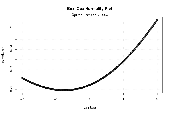
| Title produced by software | Box-Cox Normality Plot | ||||||||||||||||||||||||||||||||||||
| Date of computation | Fri, 13 Nov 2009 06:11:49 -0700 | ||||||||||||||||||||||||||||||||||||
| Cite this page as follows | Statistical Computations at FreeStatistics.org, Office for Research Development and Education, URL https://freestatistics.org/blog/index.php?v=date/2009/Nov/13/t125811810757fmgvgwm7j5uvb.htm/, Retrieved Sun, 05 May 2024 09:06:38 +0000 | ||||||||||||||||||||||||||||||||||||
| Statistical Computations at FreeStatistics.org, Office for Research Development and Education, URL https://freestatistics.org/blog/index.php?pk=56579, Retrieved Sun, 05 May 2024 09:06:38 +0000 | |||||||||||||||||||||||||||||||||||||
| QR Codes: | |||||||||||||||||||||||||||||||||||||
|
| |||||||||||||||||||||||||||||||||||||
| Original text written by user: | |||||||||||||||||||||||||||||||||||||
| IsPrivate? | No (this computation is public) | ||||||||||||||||||||||||||||||||||||
| User-defined keywords | |||||||||||||||||||||||||||||||||||||
| Estimated Impact | 108 | ||||||||||||||||||||||||||||||||||||
Tree of Dependent Computations | |||||||||||||||||||||||||||||||||||||
| Family? (F = Feedback message, R = changed R code, M = changed R Module, P = changed Parameters, D = changed Data) | |||||||||||||||||||||||||||||||||||||
| - [Box-Cox Normality Plot] [3/11/2009] [2009-11-02 22:22:24] [b98453cac15ba1066b407e146608df68] - D [Box-Cox Normality Plot] [WS6 Box cox norma...] [2009-11-13 13:11:49] [557d56ec4b06cd0135c259898de8ce95] [Current] - D [Box-Cox Normality Plot] [box cox normality ] [2009-11-13 17:03:25] [ba905ddf7cdf9ecb063c35348c4dab2e] | |||||||||||||||||||||||||||||||||||||
| Feedback Forum | |||||||||||||||||||||||||||||||||||||
Post a new message | |||||||||||||||||||||||||||||||||||||
Dataset | |||||||||||||||||||||||||||||||||||||
| Dataseries X: | |||||||||||||||||||||||||||||||||||||
10284,5 12792 12823,61538 13845,66667 15335,63636 11188,5 13633,25 12298,46667 15353,63636 12696,15385 12213,93333 13683,72727 11214,14286 13950,23077 11179,13333 11801,875 11188,82353 16456,27273 11110,0625 16530,69231 10038,41176 11681,25 11148,88235 8631 9386,444444 9764,736842 12043,75 12948,06667 10987,125 11648,3125 10633,35294 10219,3 9037,6 10296,31579 11705,41176 10681,94444 9362,947368 11306,35294 10984,45 10062,61905 8118,583333 8867,48 8346,72 8529,307692 10697,18182 8591,84 8695,607143 8125,571429 7009,758621 7883,466667 7527,645161 6763,758621 6682,333333 7855,681818 6738,88 7895,434783 6361,884615 6935,956522 8344,454545 9107,944444 | |||||||||||||||||||||||||||||||||||||
Tables (Output of Computation) | |||||||||||||||||||||||||||||||||||||
| |||||||||||||||||||||||||||||||||||||
Figures (Output of Computation) | |||||||||||||||||||||||||||||||||||||
Input Parameters & R Code | |||||||||||||||||||||||||||||||||||||
| Parameters (Session): | |||||||||||||||||||||||||||||||||||||
| Parameters (R input): | |||||||||||||||||||||||||||||||||||||
| R code (references can be found in the software module): | |||||||||||||||||||||||||||||||||||||
n <- length(x) | |||||||||||||||||||||||||||||||||||||