Free Statistics
of Irreproducible Research!
Description of Statistical Computation | |||||||||||||||||||||
|---|---|---|---|---|---|---|---|---|---|---|---|---|---|---|---|---|---|---|---|---|---|
| Author's title | |||||||||||||||||||||
| Author | *The author of this computation has been verified* | ||||||||||||||||||||
| R Software Module | rwasp_sdplot.wasp | ||||||||||||||||||||
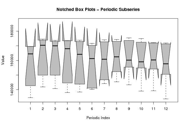
| Title produced by software | Standard Deviation Plot | ||||||||||||||||||||
| Date of computation | Thu, 12 Nov 2009 07:44:30 -0700 | ||||||||||||||||||||
| Cite this page as follows | Statistical Computations at FreeStatistics.org, Office for Research Development and Education, URL https://freestatistics.org/blog/index.php?v=date/2009/Nov/12/t1258037135661mrxovb7abtl8.htm/, Retrieved Fri, 03 May 2024 16:23:10 +0000 | ||||||||||||||||||||
| Statistical Computations at FreeStatistics.org, Office for Research Development and Education, URL https://freestatistics.org/blog/index.php?pk=56067, Retrieved Fri, 03 May 2024 16:23:10 +0000 | |||||||||||||||||||||
| QR Codes: | |||||||||||||||||||||
|
| |||||||||||||||||||||
| Original text written by user: | |||||||||||||||||||||
| IsPrivate? | No (this computation is public) | ||||||||||||||||||||
| User-defined keywords | |||||||||||||||||||||
| Estimated Impact | 124 | ||||||||||||||||||||
Tree of Dependent Computations | |||||||||||||||||||||
| Family? (F = Feedback message, R = changed R code, M = changed R Module, P = changed Parameters, D = changed Data) | |||||||||||||||||||||
| - [Standard Deviation Plot] [3/11/2009] [2009-11-02 22:09:58] [b98453cac15ba1066b407e146608df68] - PD [Standard Deviation Plot] [standard deviatio...] [2009-11-12 14:40:27] [976efdaed7598845c859b86bc2e467ce] - D [Standard Deviation Plot] [standard deviatio...] [2009-11-12 14:42:41] [976efdaed7598845c859b86bc2e467ce] - D [Standard Deviation Plot] [standard deviatio...] [2009-11-12 14:44:30] [d45d8d97b86162be82506c3c0ea6e4a6] [Current] | |||||||||||||||||||||
| Feedback Forum | |||||||||||||||||||||
Post a new message | |||||||||||||||||||||
Dataset | |||||||||||||||||||||
| Dataseries X: | |||||||||||||||||||||
168802 173276 172957 173558 173820 171663 174110 174338 175440 174922 172188 171330 169560 174579 173740 173427 172952 170305 172717 173019 173690 172439 171914 171968 169500 173898 172308 171568 164939 161275 160770 162466 160185 154836 154103 150495 142707 149962 149967 144572 143819 141070 144119 145330 143279 139063 139202 133632 134476 141859 140693 138047 138346 140167 146796 152228 155410 159032 160312 157687 160141 167421 167628 164403 163405 | |||||||||||||||||||||
Tables (Output of Computation) | |||||||||||||||||||||
| |||||||||||||||||||||
Figures (Output of Computation) | |||||||||||||||||||||
Input Parameters & R Code | |||||||||||||||||||||
| Parameters (Session): | |||||||||||||||||||||
| par1 = 50 ; par2 = 50 ; par3 = 0 ; par4 = 0 ; par5 = 0 ; par6 = Y ; par7 = Y ; | |||||||||||||||||||||
| Parameters (R input): | |||||||||||||||||||||
| par1 = 12 ; | |||||||||||||||||||||
| R code (references can be found in the software module): | |||||||||||||||||||||
par1 <- as.numeric(par1) | |||||||||||||||||||||