Free Statistics
of Irreproducible Research!
Description of Statistical Computation | |||||||||||||||||||||
|---|---|---|---|---|---|---|---|---|---|---|---|---|---|---|---|---|---|---|---|---|---|
| Author's title | |||||||||||||||||||||
| Author | *The author of this computation has been verified* | ||||||||||||||||||||
| R Software Module | rwasp_meanplot.wasp | ||||||||||||||||||||
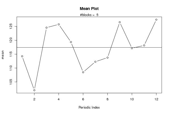
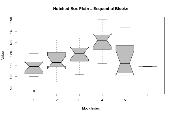
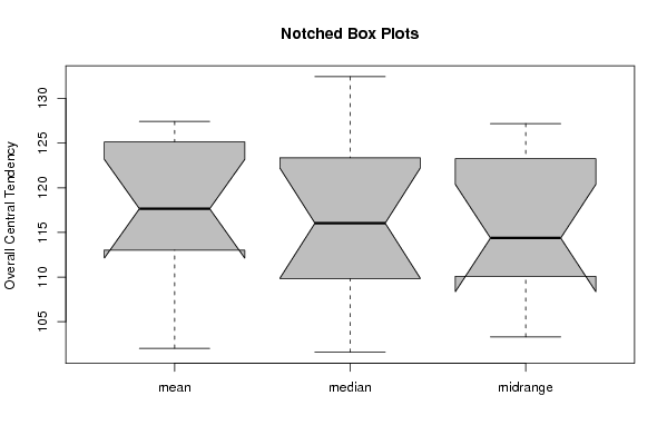
| Title produced by software | Mean Plot | ||||||||||||||||||||
| Date of computation | Wed, 11 Nov 2009 08:53:38 -0700 | ||||||||||||||||||||
| Cite this page as follows | Statistical Computations at FreeStatistics.org, Office for Research Development and Education, URL https://freestatistics.org/blog/index.php?v=date/2009/Nov/11/t1257954890kazxq61ysaetvgk.htm/, Retrieved Thu, 25 Apr 2024 18:53:15 +0000 | ||||||||||||||||||||
| Statistical Computations at FreeStatistics.org, Office for Research Development and Education, URL https://freestatistics.org/blog/index.php?pk=55720, Retrieved Thu, 25 Apr 2024 18:53:15 +0000 | |||||||||||||||||||||
| QR Codes: | |||||||||||||||||||||
|
| |||||||||||||||||||||
| Original text written by user: | |||||||||||||||||||||
| IsPrivate? | No (this computation is public) | ||||||||||||||||||||
| User-defined keywords | shwws6vr14 | ||||||||||||||||||||
| Estimated Impact | 190 | ||||||||||||||||||||
Tree of Dependent Computations | |||||||||||||||||||||
| Family? (F = Feedback message, R = changed R code, M = changed R Module, P = changed Parameters, D = changed Data) | |||||||||||||||||||||
| - [Mean Plot] [3/11/2009] [2009-11-02 22:07:54] [b98453cac15ba1066b407e146608df68] - R PD [Mean Plot] [] [2009-11-11 15:53:38] [4407d6264e55b051ec65750e6dca2820] [Current] | |||||||||||||||||||||
| Feedback Forum | |||||||||||||||||||||
Post a new message | |||||||||||||||||||||
Dataset | |||||||||||||||||||||
| Dataseries X: | |||||||||||||||||||||
100 87,14054095 112,0054296 112,312101 109,474134 104,9746116 100,4926851 104,2154743 120,1768388 112,1028355 108,1481575 116,802197 102,1699512 95,15358705 120,6707808 111,5234277 119,9669448 113,3697401 110,0717661 111,5567342 132,424212 107,900558 122,1626615 124,3992258 110,4450505 101,5874013 122,3203962 125,2582826 125,4411543 108,9902468 118,9243879 116,7242723 134,1724901 116,8530994 124,5732995 130,9914031 123,4239103 111,4536725 124,5135991 139,2589613 129,8596099 112,3460359 131,381655 133,0004776 134,3220552 144,2379719 134,1278719 150,1891559 140,722563 114,8389975 143,1973003 140,2738676 112,1248303 102,8951536 100,5090242 103,3513901 111,4134533 104,5887587 101,7840983 114,7007441 108,7426474 | |||||||||||||||||||||
Tables (Output of Computation) | |||||||||||||||||||||
| |||||||||||||||||||||
Figures (Output of Computation) | |||||||||||||||||||||
Input Parameters & R Code | |||||||||||||||||||||
| Parameters (Session): | |||||||||||||||||||||
| par1 = 12 ; | |||||||||||||||||||||
| Parameters (R input): | |||||||||||||||||||||
| par1 = 12 ; | |||||||||||||||||||||
| R code (references can be found in the software module): | |||||||||||||||||||||
par1 <- as.numeric(par1) | |||||||||||||||||||||