Free Statistics
of Irreproducible Research!
Description of Statistical Computation | |||||||||||||||||||||||||||||||||||||||||||||||||||||||||||||||||
|---|---|---|---|---|---|---|---|---|---|---|---|---|---|---|---|---|---|---|---|---|---|---|---|---|---|---|---|---|---|---|---|---|---|---|---|---|---|---|---|---|---|---|---|---|---|---|---|---|---|---|---|---|---|---|---|---|---|---|---|---|---|---|---|---|---|
| Author's title | |||||||||||||||||||||||||||||||||||||||||||||||||||||||||||||||||
| Author | *The author of this computation has been verified* | ||||||||||||||||||||||||||||||||||||||||||||||||||||||||||||||||
| R Software Module | rwasp_edabi.wasp | ||||||||||||||||||||||||||||||||||||||||||||||||||||||||||||||||
| Title produced by software | Bivariate Explorative Data Analysis | ||||||||||||||||||||||||||||||||||||||||||||||||||||||||||||||||
| Date of computation | Wed, 11 Nov 2009 08:20:29 -0700 | ||||||||||||||||||||||||||||||||||||||||||||||||||||||||||||||||
| Cite this page as follows | Statistical Computations at FreeStatistics.org, Office for Research Development and Education, URL https://freestatistics.org/blog/index.php?v=date/2009/Nov/11/t12579529845pev3iyd85k4jym.htm/, Retrieved Wed, 24 Apr 2024 05:32:59 +0000 | ||||||||||||||||||||||||||||||||||||||||||||||||||||||||||||||||
| Statistical Computations at FreeStatistics.org, Office for Research Development and Education, URL https://freestatistics.org/blog/index.php?pk=55681, Retrieved Wed, 24 Apr 2024 05:32:59 +0000 | |||||||||||||||||||||||||||||||||||||||||||||||||||||||||||||||||
| QR Codes: | |||||||||||||||||||||||||||||||||||||||||||||||||||||||||||||||||
|
| |||||||||||||||||||||||||||||||||||||||||||||||||||||||||||||||||
| Original text written by user: | |||||||||||||||||||||||||||||||||||||||||||||||||||||||||||||||||
| IsPrivate? | No (this computation is public) | ||||||||||||||||||||||||||||||||||||||||||||||||||||||||||||||||
| User-defined keywords | |||||||||||||||||||||||||||||||||||||||||||||||||||||||||||||||||
| Estimated Impact | 126 | ||||||||||||||||||||||||||||||||||||||||||||||||||||||||||||||||
Tree of Dependent Computations | |||||||||||||||||||||||||||||||||||||||||||||||||||||||||||||||||
| Family? (F = Feedback message, R = changed R code, M = changed R Module, P = changed Parameters, D = changed Data) | |||||||||||||||||||||||||||||||||||||||||||||||||||||||||||||||||
| - [Bagplot] [3/11/2009] [2009-11-02 21:51:11] [b98453cac15ba1066b407e146608df68] - RMPD [Bivariate Explorative Data Analysis] [WS6_bivariateEDA] [2009-11-11 15:20:29] [7a6d96edf94be87996de99db5f42363b] [Current] | |||||||||||||||||||||||||||||||||||||||||||||||||||||||||||||||||
| Feedback Forum | |||||||||||||||||||||||||||||||||||||||||||||||||||||||||||||||||
Post a new message | |||||||||||||||||||||||||||||||||||||||||||||||||||||||||||||||||
Dataset | |||||||||||||||||||||||||||||||||||||||||||||||||||||||||||||||||
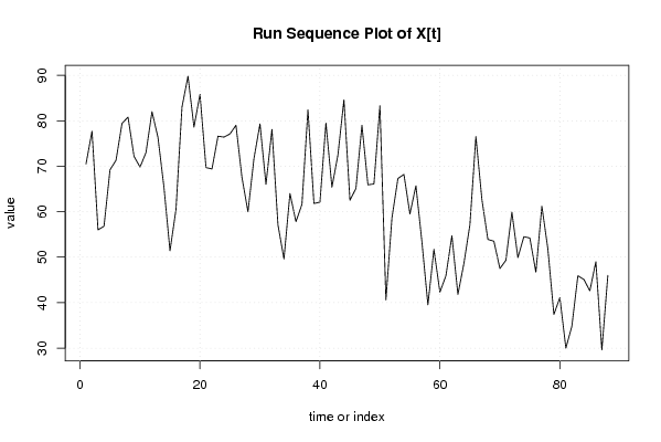
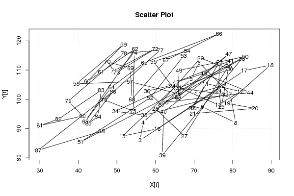
| Dataseries X: | |||||||||||||||||||||||||||||||||||||||||||||||||||||||||||||||||
70,5 77,7 56,0 56,8 69,2 71,3 79,4 80,8 72,2 69,8 73,0 82,0 76,3 65,3 51,4 60,5 83,0 89,8 78,6 85,8 69,7 69,4 76,6 76,4 77,1 79,0 67,5 60,0 71,7 79,3 66,0 78,1 57,1 49,6 64,0 57,8 61,6 82,4 61,8 62,1 79,5 65,4 72,5 84,6 62,5 65,1 79,0 65,9 66,1 83,3 40,6 58,6 67,3 68,2 59,5 65,7 53,4 39,5 51,7 42,3 45,9 54,7 41,8 48,6 57,1 76,5 62,7 53,9 53,5 47,5 49,3 59,9 49,9 54,5 54,2 46,7 61,2 51,8 37,4 41,1 30,0 34,8 45,9 45,1 42,6 49,0 29,6 46,0 | |||||||||||||||||||||||||||||||||||||||||||||||||||||||||||||||||
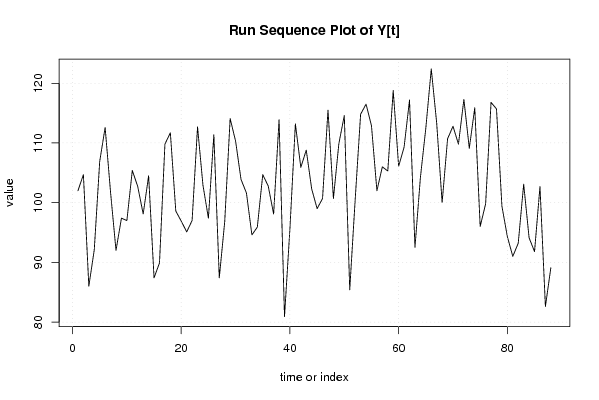
| Dataseries Y: | |||||||||||||||||||||||||||||||||||||||||||||||||||||||||||||||||
102,0 104,7 86,0 92,1 106,9 112,6 101,7 92,0 97,4 97,0 105,4 102,7 98,1 104,5 87,4 89,9 109,8 111,7 98,6 96,9 95,1 97,0 112,7 102,9 97,4 111,4 87,4 96,8 114,1 110,3 103,9 101,6 94,6 95,9 104,7 102,8 98,1 113,9 80,9 95,7 113,2 105,9 108,8 102,3 99,0 100,7 115,5 100,7 109,9 114,6 85,4 100,5 114,8 116,5 112,9 102,0 106,0 105,3 118,8 106,1 109,3 117,2 92,5 104,2 112,5 122,4 113,3 100,0 110,7 112,8 109,8 117,3 109,1 115,9 96,0 99,8 116,8 115,7 99,4 94,3 91,0 93,2 103,1 94,1 91,8 102,7 82,6 89,1 | |||||||||||||||||||||||||||||||||||||||||||||||||||||||||||||||||
Tables (Output of Computation) | |||||||||||||||||||||||||||||||||||||||||||||||||||||||||||||||||
| |||||||||||||||||||||||||||||||||||||||||||||||||||||||||||||||||
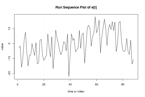
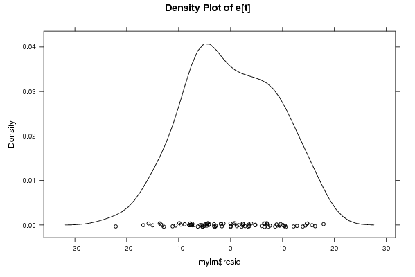
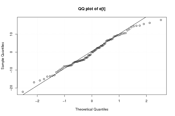
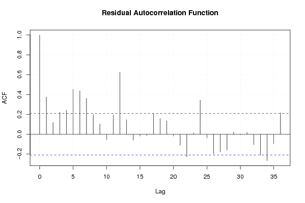
Figures (Output of Computation) | |||||||||||||||||||||||||||||||||||||||||||||||||||||||||||||||||
Input Parameters & R Code | |||||||||||||||||||||||||||||||||||||||||||||||||||||||||||||||||
| Parameters (Session): | |||||||||||||||||||||||||||||||||||||||||||||||||||||||||||||||||
| par1 = 0 ; par2 = 36 ; | |||||||||||||||||||||||||||||||||||||||||||||||||||||||||||||||||
| Parameters (R input): | |||||||||||||||||||||||||||||||||||||||||||||||||||||||||||||||||
| par1 = 0 ; par2 = 36 ; | |||||||||||||||||||||||||||||||||||||||||||||||||||||||||||||||||
| R code (references can be found in the software module): | |||||||||||||||||||||||||||||||||||||||||||||||||||||||||||||||||
par1 <- as.numeric(par1) | |||||||||||||||||||||||||||||||||||||||||||||||||||||||||||||||||