Free Statistics
of Irreproducible Research!
Description of Statistical Computation | |||||||||||||||||||||
|---|---|---|---|---|---|---|---|---|---|---|---|---|---|---|---|---|---|---|---|---|---|
| Author's title | |||||||||||||||||||||
| Author | *The author of this computation has been verified* | ||||||||||||||||||||
| R Software Module | rwasp_meanplot.wasp | ||||||||||||||||||||
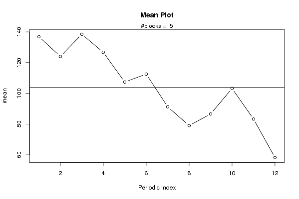
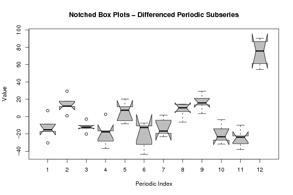
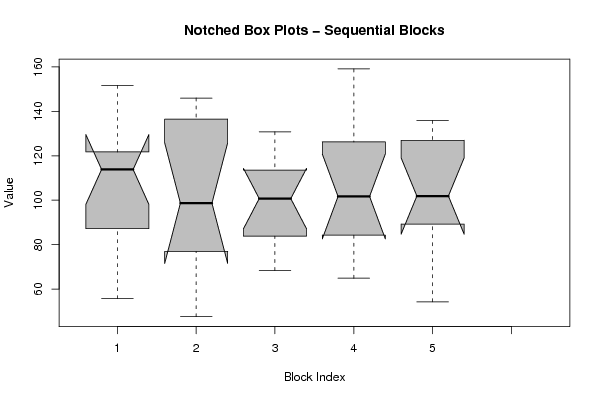
| Title produced by software | Mean Plot | ||||||||||||||||||||
| Date of computation | Wed, 11 Nov 2009 07:55:56 -0700 | ||||||||||||||||||||
| Cite this page as follows | Statistical Computations at FreeStatistics.org, Office for Research Development and Education, URL https://freestatistics.org/blog/index.php?v=date/2009/Nov/11/t12579516947sf1q72r8ymc2j6.htm/, Retrieved Fri, 19 Apr 2024 04:42:24 +0000 | ||||||||||||||||||||
| Statistical Computations at FreeStatistics.org, Office for Research Development and Education, URL https://freestatistics.org/blog/index.php?pk=55655, Retrieved Fri, 19 Apr 2024 04:42:24 +0000 | |||||||||||||||||||||
| QR Codes: | |||||||||||||||||||||
|
| |||||||||||||||||||||
| Original text written by user: | |||||||||||||||||||||
| IsPrivate? | No (this computation is public) | ||||||||||||||||||||
| User-defined keywords | ShwWs6.6 | ||||||||||||||||||||
| Estimated Impact | 136 | ||||||||||||||||||||
Tree of Dependent Computations | |||||||||||||||||||||
| Family? (F = Feedback message, R = changed R code, M = changed R Module, P = changed Parameters, D = changed Data) | |||||||||||||||||||||
| - [Bagplot] [3/11/2009] [2009-11-02 21:51:11] [b98453cac15ba1066b407e146608df68] - RMPD [Mean Plot] [Ws6.6 Mean Plot] [2009-11-11 14:55:56] [51108381f3361ca8af49c4f74052c840] [Current] | |||||||||||||||||||||
| Feedback Forum | |||||||||||||||||||||
Post a new message | |||||||||||||||||||||
Dataset | |||||||||||||||||||||
| Dataseries X: | |||||||||||||||||||||
151,7 121,3 133,0 119,6 122,2 117,4 106,7 87,5 81,0 110,3 87,0 55,7 146,0 137,5 138,5 135,6 107,3 99,0 91,4 68,4 82,6 98,4 71,3 47,6 130,8 113,6 125,7 113,6 97,1 104,4 91,8 75,1 89,2 110,2 78,4 68,4 122,8 129,7 159,1 139,0 102,2 113,6 81,5 77,4 87,6 101,2 87,2 64,9 133,1 118,0 135,9 125,7 108,0 128,3 84,7 86,4 92,2 95,8 92,3 54,3 | |||||||||||||||||||||
Tables (Output of Computation) | |||||||||||||||||||||
| |||||||||||||||||||||
Figures (Output of Computation) | |||||||||||||||||||||
Input Parameters & R Code | |||||||||||||||||||||
| Parameters (Session): | |||||||||||||||||||||
| par1 = 12 ; | |||||||||||||||||||||
| Parameters (R input): | |||||||||||||||||||||
| par1 = 12 ; | |||||||||||||||||||||
| R code (references can be found in the software module): | |||||||||||||||||||||
par1 <- as.numeric(par1) | |||||||||||||||||||||