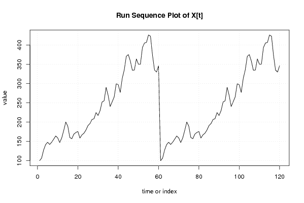
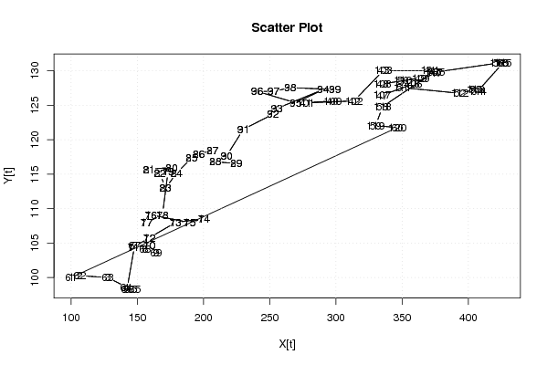
100,00
106,54
127,63
141,72
147,95
142,16
147,95
155,82
164,13
159,16
147,14
159,16
178,85
200,44
189,43
160,16
157,02
168,91
173,19
175,83
158,78
166,96
171,24
179,55
191,00
196,41
206,80
208,94
224,86
217,31
229,96
252,36
255,25
290,37
269,67
240,53
252,86
265,51
299,31
297,42
277,09
313,59
335,75
370,67
375,33
358,65
334,80
335,05
364,07
350,47
350,16
393,46
405,29
406,86
426,12
422,97
373,63
335,18
329,89
346,32
100,00
106,54
127,63
141,72
147,95
142,16
147,95
155,82
164,13
159,16
147,14
159,16
178,85
200,44
189,43
160,16
157,02
168,91
173,19
175,83
158,78
166,96
171,24
179,55
191,00
196,41
206,80
208,94
224,86
217,31
229,96
252,36
255,25
290,37
269,67
240,53
252,86
265,51
299,31
297,42
277,09
313,59
335,75
370,67
375,33
358,65
334,80
335,05
364,07
350,47
350,16
393,46
405,29
406,86
426,12
422,97
373,63
335,18
329,89
346,32 |
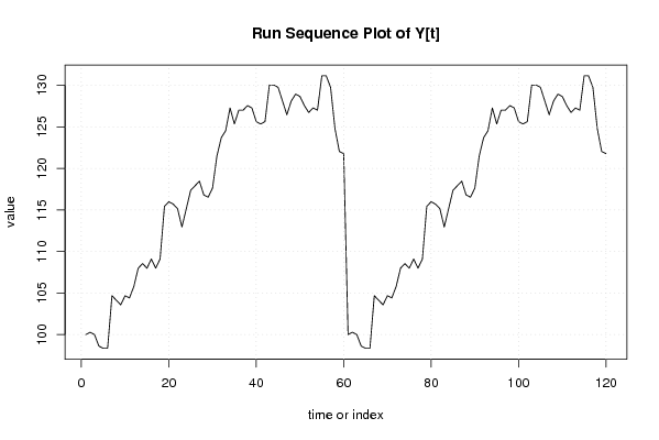
100,00
100,28
100,00
98,62
98,35
98,35
104,68
104,13
103,58
104,68
104,41
105,79
107,99
108,54
107,99
109,09
107,99
109,09
115,43
115,98
115,70
115,15
112,95
115,15
117,36
117,91
118,46
116,80
116,53
117,63
121,49
123,69
124,52
127,27
125,34
127,00
127,00
127,55
127,27
125,62
125,34
125,62
130,03
130,03
129,75
128,10
126,45
128,10
128,93
128,65
127,55
126,72
127,27
127,00
131,13
131,13
129,75
124,79
122,04
121,76
100,00
100,28
100,00
98,62
98,35
98,35
104,68
104,13
103,58
104,68
104,41
105,79
107,99
108,54
107,99
109,09
107,99
109,09
115,43
115,98
115,70
115,15
112,95
115,15
117,36
117,91
118,46
116,80
116,53
117,63
121,49
123,69
124,52
127,27
125,34
127,00
127,00
127,55
127,27
125,62
125,34
125,62
130,03
130,03
129,75
128,10
126,45
128,10
128,93
128,65
127,55
126,72
127,27
127,00
131,13
131,13
129,75
124,79
122,04
121,76 |