Free Statistics
of Irreproducible Research!
Description of Statistical Computation | |||||||||||||||||||||||||||||||||||||||||||||
|---|---|---|---|---|---|---|---|---|---|---|---|---|---|---|---|---|---|---|---|---|---|---|---|---|---|---|---|---|---|---|---|---|---|---|---|---|---|---|---|---|---|---|---|---|---|
| Author's title | |||||||||||||||||||||||||||||||||||||||||||||
| Author | *The author of this computation has been verified* | ||||||||||||||||||||||||||||||||||||||||||||
| R Software Module | rwasp_boxcoxlin.wasp | ||||||||||||||||||||||||||||||||||||||||||||
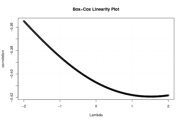
| Title produced by software | Box-Cox Linearity Plot | ||||||||||||||||||||||||||||||||||||||||||||
| Date of computation | Wed, 11 Nov 2009 04:42:34 -0700 | ||||||||||||||||||||||||||||||||||||||||||||
| Cite this page as follows | Statistical Computations at FreeStatistics.org, Office for Research Development and Education, URL https://freestatistics.org/blog/index.php?v=date/2009/Nov/11/t1257939795qok4je4cbl13x0v.htm/, Retrieved Thu, 18 Apr 2024 21:20:30 +0000 | ||||||||||||||||||||||||||||||||||||||||||||
| Statistical Computations at FreeStatistics.org, Office for Research Development and Education, URL https://freestatistics.org/blog/index.php?pk=55505, Retrieved Thu, 18 Apr 2024 21:20:30 +0000 | |||||||||||||||||||||||||||||||||||||||||||||
| QR Codes: | |||||||||||||||||||||||||||||||||||||||||||||
|
| |||||||||||||||||||||||||||||||||||||||||||||
| Original text written by user: | |||||||||||||||||||||||||||||||||||||||||||||
| IsPrivate? | No (this computation is public) | ||||||||||||||||||||||||||||||||||||||||||||
| User-defined keywords | |||||||||||||||||||||||||||||||||||||||||||||
| Estimated Impact | 182 | ||||||||||||||||||||||||||||||||||||||||||||
Tree of Dependent Computations | |||||||||||||||||||||||||||||||||||||||||||||
| Family? (F = Feedback message, R = changed R code, M = changed R Module, P = changed Parameters, D = changed Data) | |||||||||||||||||||||||||||||||||||||||||||||
| - [Box-Cox Linearity Plot] [3/11/2009] [2009-11-02 21:47:57] [b98453cac15ba1066b407e146608df68] - D [Box-Cox Linearity Plot] [] [2009-11-11 11:42:34] [d41d8cd98f00b204e9800998ecf8427e] [Current] | |||||||||||||||||||||||||||||||||||||||||||||
| Feedback Forum | |||||||||||||||||||||||||||||||||||||||||||||
Post a new message | |||||||||||||||||||||||||||||||||||||||||||||
Dataset | |||||||||||||||||||||||||||||||||||||||||||||
| Dataseries X: | |||||||||||||||||||||||||||||||||||||||||||||
100,00 127,27 109,09 136,36 100,00 118,18 136,36 100,00 127,27 118,18 136,36 145,45 154,55 100,00 145,45 118,18 154,55 145,45 154,55 172,73 163,64 172,73 145,45 136,36 145,45 145,45 154,55 181,82 181,82 172,73 154,55 163,64 172,73 154,55 181,82 190,91 218,18 227,27 227,27 236,36 200,00 227,27 254,55 254,55 263,64 272,73 281,82 263,64 245,45 200,00 227,27 209,09 236,36 209,09 200,00 163,64 163,64 181,82 145,45 163,64 | |||||||||||||||||||||||||||||||||||||||||||||
| Dataseries Y: | |||||||||||||||||||||||||||||||||||||||||||||
100,00 98,86 96,87 103,18 104,66 103,74 103,87 98,10 98,91 109,43 104,89 88,63 97,03 93,79 97,61 98,17 96,31 97,82 87,52 85,71 89,15 90,65 92,74 80,00 84,33 93,26 115,89 105,21 94,23 106,12 94,41 101,30 98,43 107,94 102,82 92,33 97,48 88,37 92,50 81,48 92,55 98,96 77,28 91,01 81,21 88,41 96,02 91,59 86,30 86,37 105,41 76,73 93,26 95,02 84,32 93,24 89,81 111,66 103,23 103,21 | |||||||||||||||||||||||||||||||||||||||||||||
Tables (Output of Computation) | |||||||||||||||||||||||||||||||||||||||||||||
| |||||||||||||||||||||||||||||||||||||||||||||
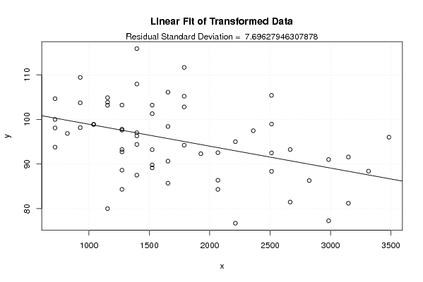
Figures (Output of Computation) | |||||||||||||||||||||||||||||||||||||||||||||
Input Parameters & R Code | |||||||||||||||||||||||||||||||||||||||||||||
| Parameters (Session): | |||||||||||||||||||||||||||||||||||||||||||||
| Parameters (R input): | |||||||||||||||||||||||||||||||||||||||||||||
| R code (references can be found in the software module): | |||||||||||||||||||||||||||||||||||||||||||||
n <- length(x) | |||||||||||||||||||||||||||||||||||||||||||||