Free Statistics
of Irreproducible Research!
Description of Statistical Computation | |||||||||||||||||||||||||||||||||||||||||||||||||||||||||||||||||||||||||||||||||||||||||||||||||||||||||||||||||||||||||||||||||||||||||||||
|---|---|---|---|---|---|---|---|---|---|---|---|---|---|---|---|---|---|---|---|---|---|---|---|---|---|---|---|---|---|---|---|---|---|---|---|---|---|---|---|---|---|---|---|---|---|---|---|---|---|---|---|---|---|---|---|---|---|---|---|---|---|---|---|---|---|---|---|---|---|---|---|---|---|---|---|---|---|---|---|---|---|---|---|---|---|---|---|---|---|---|---|---|---|---|---|---|---|---|---|---|---|---|---|---|---|---|---|---|---|---|---|---|---|---|---|---|---|---|---|---|---|---|---|---|---|---|---|---|---|---|---|---|---|---|---|---|---|---|---|---|---|
| Author's title | |||||||||||||||||||||||||||||||||||||||||||||||||||||||||||||||||||||||||||||||||||||||||||||||||||||||||||||||||||||||||||||||||||||||||||||
| Author | *Unverified author* | ||||||||||||||||||||||||||||||||||||||||||||||||||||||||||||||||||||||||||||||||||||||||||||||||||||||||||||||||||||||||||||||||||||||||||||
| R Software Module | rwasp_notchedbox1.wasp | ||||||||||||||||||||||||||||||||||||||||||||||||||||||||||||||||||||||||||||||||||||||||||||||||||||||||||||||||||||||||||||||||||||||||||||
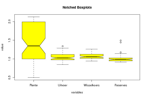
| Title produced by software | Notched Boxplots | ||||||||||||||||||||||||||||||||||||||||||||||||||||||||||||||||||||||||||||||||||||||||||||||||||||||||||||||||||||||||||||||||||||||||||||
| Date of computation | Wed, 11 Nov 2009 03:39:32 -0700 | ||||||||||||||||||||||||||||||||||||||||||||||||||||||||||||||||||||||||||||||||||||||||||||||||||||||||||||||||||||||||||||||||||||||||||||
| Cite this page as follows | Statistical Computations at FreeStatistics.org, Office for Research Development and Education, URL https://freestatistics.org/blog/index.php?v=date/2009/Nov/11/t1257936022eky2ddtgquqlww5.htm/, Retrieved Sat, 20 Apr 2024 12:38:40 +0000 | ||||||||||||||||||||||||||||||||||||||||||||||||||||||||||||||||||||||||||||||||||||||||||||||||||||||||||||||||||||||||||||||||||||||||||||
| Statistical Computations at FreeStatistics.org, Office for Research Development and Education, URL https://freestatistics.org/blog/index.php?pk=55476, Retrieved Sat, 20 Apr 2024 12:38:40 +0000 | |||||||||||||||||||||||||||||||||||||||||||||||||||||||||||||||||||||||||||||||||||||||||||||||||||||||||||||||||||||||||||||||||||||||||||||
| QR Codes: | |||||||||||||||||||||||||||||||||||||||||||||||||||||||||||||||||||||||||||||||||||||||||||||||||||||||||||||||||||||||||||||||||||||||||||||
|
| |||||||||||||||||||||||||||||||||||||||||||||||||||||||||||||||||||||||||||||||||||||||||||||||||||||||||||||||||||||||||||||||||||||||||||||
| Original text written by user: | |||||||||||||||||||||||||||||||||||||||||||||||||||||||||||||||||||||||||||||||||||||||||||||||||||||||||||||||||||||||||||||||||||||||||||||
| IsPrivate? | No (this computation is public) | ||||||||||||||||||||||||||||||||||||||||||||||||||||||||||||||||||||||||||||||||||||||||||||||||||||||||||||||||||||||||||||||||||||||||||||
| User-defined keywords | |||||||||||||||||||||||||||||||||||||||||||||||||||||||||||||||||||||||||||||||||||||||||||||||||||||||||||||||||||||||||||||||||||||||||||||
| Estimated Impact | 211 | ||||||||||||||||||||||||||||||||||||||||||||||||||||||||||||||||||||||||||||||||||||||||||||||||||||||||||||||||||||||||||||||||||||||||||||
Tree of Dependent Computations | |||||||||||||||||||||||||||||||||||||||||||||||||||||||||||||||||||||||||||||||||||||||||||||||||||||||||||||||||||||||||||||||||||||||||||||
| Family? (F = Feedback message, R = changed R code, M = changed R Module, P = changed Parameters, D = changed Data) | |||||||||||||||||||||||||||||||||||||||||||||||||||||||||||||||||||||||||||||||||||||||||||||||||||||||||||||||||||||||||||||||||||||||||||||
| - [Notched Boxplots] [] [2009-11-11 10:39:32] [e76c6d261190c0179bc6006a5cdb804c] [Current] | |||||||||||||||||||||||||||||||||||||||||||||||||||||||||||||||||||||||||||||||||||||||||||||||||||||||||||||||||||||||||||||||||||||||||||||
| Feedback Forum | |||||||||||||||||||||||||||||||||||||||||||||||||||||||||||||||||||||||||||||||||||||||||||||||||||||||||||||||||||||||||||||||||||||||||||||
Post a new message | |||||||||||||||||||||||||||||||||||||||||||||||||||||||||||||||||||||||||||||||||||||||||||||||||||||||||||||||||||||||||||||||||||||||||||||
Dataset | |||||||||||||||||||||||||||||||||||||||||||||||||||||||||||||||||||||||||||||||||||||||||||||||||||||||||||||||||||||||||||||||||||||||||||||
| Dataseries X: | |||||||||||||||||||||||||||||||||||||||||||||||||||||||||||||||||||||||||||||||||||||||||||||||||||||||||||||||||||||||||||||||||||||||||||||
1 1 1 1 1 1.002738004 1.04011209 0.98537037 1 0.977400242 1.073498799 0.950833333 1 0.937227883 1.050360288 0.943425926 1 0.897212622 1.041953563 0.914444444 1 0.874343552 1.05692554 0.941111111 1 1.072955474 1.035868695 0.917222222 1 1.000869653 1.016333066 0.926203704 1 0.96556174 0.973979183 0.978148148 1 1.042826204 0.963730985 0.946388889 1 0.912187486 0.984147318 0.930740741 1 0.849544414 0.981265012 0.973333333 1 1.077365456 0.961969576 0.978981481 1 0.99569662 0.943634908 1.001944444 1.105 1.071081512 0.949239392 0.941388889 1.125 1.012180753 0.969015212 1.009351852 1.125 0.982735985 0.955804644 1.008888889 1.225 0.995993985 0.962369896 1.012407407 1.25 1.182301719 0.982465973 1.023981481 1.25 0.963351138 1.022417934 0.973425926 1.32 1.090685174 1.012810248 0.950925926 1.375 1.11065353 1.015532426 0.96287037 1.465 0.986068719 1.02570056 0.994444444 1.5 0.9069864 1.01897518 0.950277778 1.585 1.092093451 1.00968775 0.915092593 1.625 1.118323309 1.031305044 0.944814815 1.695 1.119956012 1.057886309 0.944537037 1.75 0.973080031 1.040752602 0.964444444 1.75 1.061773419 1.046757406 0.9775 1.825 1.042130482 1.060208167 0.941296296 1.875 1.197910588 1.082145717 0.932037037 1.875 1.043280668 1.081745396 0.936759259 1.95 1.112712644 1.074379504 0.923425926 2 1.169509403 1.098158527 0.959259259 2 1.101945779 1.090632506 0.938240741 2 0.995073836 1.112570056 0.987685185 2 1.111674671 1.139071257 1.007685185 2 1.243323309 1.175660528 0.999444444 2 1.159404596 1.166533227 1.038148148 2 1.00304098 1.178382706 1.040925926 2 1.172993626 1.180784628 1.063240741 2 1.187446699 1.243154524 1.028333333 2 1.199245927 1.261008807 1.020277778 2 1.287776606 1.245556445 0.996944444 2 1.197512231 1.245236189 0.979351852 2.09 1.340909601 1.262610088 1.005462963 2.125 1.256390547 1.198959167 0.979166667 2.125 1.025298487 1.150440352 0.988888889 1.985 1.278485345 1.066613291 1.011666667 1.71 1.252384533 1.0193755 1.090833333 1.375 1.001066026 1.076781425 1.040833333 1.155 0.918662193 1.059967974 1.143240741 1 0.8939921 1.023618895 1.175833333 0.83 0.922735536 1.044835869 1.130925926 0.655 0.994714754 1.056044836 1.117222222 0.545 0.933782935 1.092874299 1.118981481 0.5 0.908742538 1.122177742 1.101296296 0.5 1.024064141 1.127942354 1.091944444 0.5 0.98581624 1.142353883 1.441388889 0.5 0.888549755 1.165892714 1.493981481 | |||||||||||||||||||||||||||||||||||||||||||||||||||||||||||||||||||||||||||||||||||||||||||||||||||||||||||||||||||||||||||||||||||||||||||||
Tables (Output of Computation) | |||||||||||||||||||||||||||||||||||||||||||||||||||||||||||||||||||||||||||||||||||||||||||||||||||||||||||||||||||||||||||||||||||||||||||||
| |||||||||||||||||||||||||||||||||||||||||||||||||||||||||||||||||||||||||||||||||||||||||||||||||||||||||||||||||||||||||||||||||||||||||||||
Figures (Output of Computation) | |||||||||||||||||||||||||||||||||||||||||||||||||||||||||||||||||||||||||||||||||||||||||||||||||||||||||||||||||||||||||||||||||||||||||||||
Input Parameters & R Code | |||||||||||||||||||||||||||||||||||||||||||||||||||||||||||||||||||||||||||||||||||||||||||||||||||||||||||||||||||||||||||||||||||||||||||||
| Parameters (Session): | |||||||||||||||||||||||||||||||||||||||||||||||||||||||||||||||||||||||||||||||||||||||||||||||||||||||||||||||||||||||||||||||||||||||||||||
| par1 = yellow ; | |||||||||||||||||||||||||||||||||||||||||||||||||||||||||||||||||||||||||||||||||||||||||||||||||||||||||||||||||||||||||||||||||||||||||||||
| Parameters (R input): | |||||||||||||||||||||||||||||||||||||||||||||||||||||||||||||||||||||||||||||||||||||||||||||||||||||||||||||||||||||||||||||||||||||||||||||
| par1 = yellow ; | |||||||||||||||||||||||||||||||||||||||||||||||||||||||||||||||||||||||||||||||||||||||||||||||||||||||||||||||||||||||||||||||||||||||||||||
| R code (references can be found in the software module): | |||||||||||||||||||||||||||||||||||||||||||||||||||||||||||||||||||||||||||||||||||||||||||||||||||||||||||||||||||||||||||||||||||||||||||||
z <- as.data.frame(t(y)) | |||||||||||||||||||||||||||||||||||||||||||||||||||||||||||||||||||||||||||||||||||||||||||||||||||||||||||||||||||||||||||||||||||||||||||||