Free Statistics
of Irreproducible Research!
Description of Statistical Computation | |||||||||||||||||||||
|---|---|---|---|---|---|---|---|---|---|---|---|---|---|---|---|---|---|---|---|---|---|
| Author's title | |||||||||||||||||||||
| Author | *The author of this computation has been verified* | ||||||||||||||||||||
| R Software Module | rwasp_sdplot.wasp | ||||||||||||||||||||
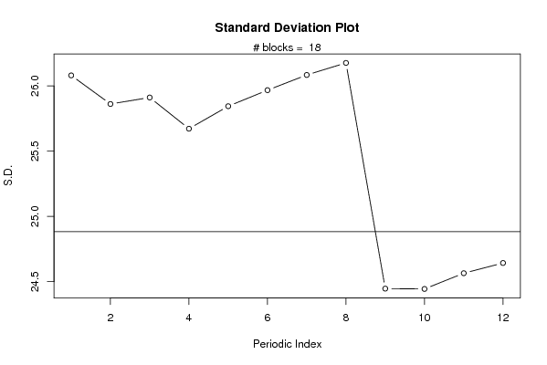
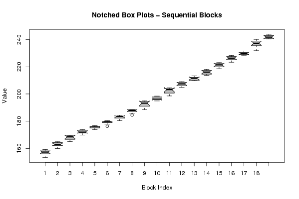
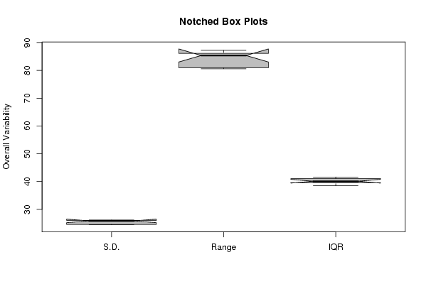
| Title produced by software | Standard Deviation Plot | ||||||||||||||||||||
| Date of computation | Wed, 11 Nov 2009 03:35:01 -0700 | ||||||||||||||||||||
| Cite this page as follows | Statistical Computations at FreeStatistics.org, Office for Research Development and Education, URL https://freestatistics.org/blog/index.php?v=date/2009/Nov/11/t1257935730c0g979gy18hvfm2.htm/, Retrieved Mon, 30 Jun 2025 23:14:27 +0000 | ||||||||||||||||||||
| Statistical Computations at FreeStatistics.org, Office for Research Development and Education, URL https://freestatistics.org/blog/index.php?pk=55471, Retrieved Mon, 30 Jun 2025 23:14:27 +0000 | |||||||||||||||||||||
| QR Codes: | |||||||||||||||||||||
|
| |||||||||||||||||||||
| Original text written by user: | |||||||||||||||||||||
| IsPrivate? | No (this computation is public) | ||||||||||||||||||||
| User-defined keywords | |||||||||||||||||||||
| Estimated Impact | 273 | ||||||||||||||||||||
Tree of Dependent Computations | |||||||||||||||||||||
| Family? (F = Feedback message, R = changed R code, M = changed R Module, P = changed Parameters, D = changed Data) | |||||||||||||||||||||
| - [Standard Deviation Plot] [3/11/2009] [2009-11-02 22:09:58] [b98453cac15ba1066b407e146608df68] - PD [Standard Deviation Plot] [ws6 range plot] [2009-11-06 16:04:51] [8b1aef4e7013bd33fbc2a5833375c5f5] - [Standard Deviation Plot] [] [2009-11-11 10:35:01] [2a6f24d4847085573f343c759dfbabef] [Current] | |||||||||||||||||||||
| Feedback Forum | |||||||||||||||||||||
Post a new message | |||||||||||||||||||||
Dataset | |||||||||||||||||||||
| Dataseries X: | |||||||||||||||||||||
153.3 154.5 155.2 156.9 157 157.4 157.2 157.5 158 158.5 159 159.3 160 160.8 161.9 162.5 162.7 162.8 162.9 163 164 164.7 164.8 164.9 165 165.8 166.1 167.2 167.7 168.3 168.6 168.9 169.1 169.5 169.6 169.7 169.8 170.4 170.9 171.9 171.9 172 172 172.4 173 173.7 173.8 173.8 173.9 174.6 175 175.9 176 175.1 175.6 175.9 176.7 176.1 176.1 176.2 176.3 177.8 178.5 179.4 179.5 179.6 179.7 179.7 179.8 179.9 180.2 180.4 180.4 181.3 181.9 182.5 182.7 183.1 183.6 183.7 183.8 183.9 184.1 184.4 184.5 185.9 186.6 187.6 187.8 187.9 188 188.3 188.4 188.5 188.5 188.6 188.6 189.4 190 191.9 192.5 193 193.5 193.9 194.2 194.9 194.9 194.9 194.9 195.5 196 196.2 196.2 196.2 196.2 197 197.7 198 198.2 198.5 198.6 199.5 200 201.3 202.2 202.9 203.5 203.5 204 204.1 204.3 204.5 204.8 205.1 205.7 206.5 206.9 207.1 207.8 208 208.5 208.6 209 209.1 209.7 209.8 209.9 210 210.8 211.4 211.7 212 212.2 212.4 212.9 213.4 213.7 214 214.3 214.8 215 215.9 216.4 216.9 217.2 217.5 217.9 218.1 218.6 218.9 219.3 220.4 220.9 221 221.8 222 222.2 222.5 222.9 223.1 223.4 224 225.1 225.5 225.9 226.3 226.5 227 227.3 227.8 228.1 228.4 228.5 228.8 229 229.1 229.3 229.6 229.9 230 230.2 230.8 231 231.7 231.9 233 235.1 236 236.9 237.1 237.5 238.2 238.9 239.1 240 240.2 240.5 240.7 241.1 241.4 242.2 242.9 243.2 243.9 | |||||||||||||||||||||
Tables (Output of Computation) | |||||||||||||||||||||
| |||||||||||||||||||||
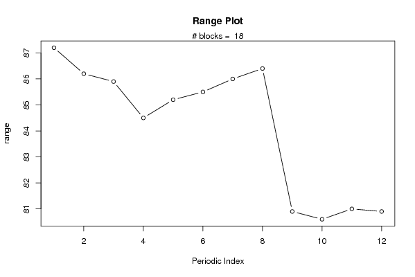
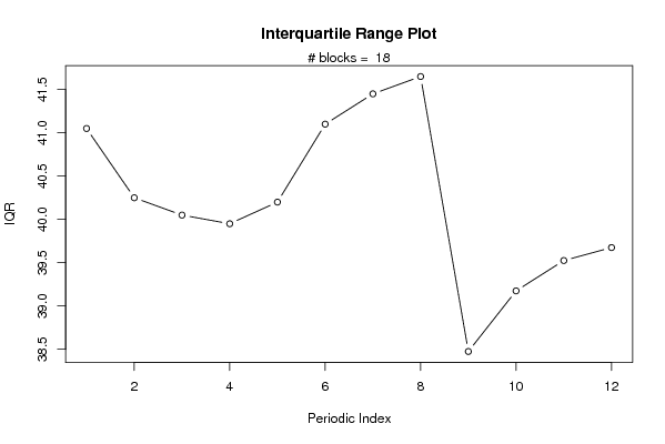
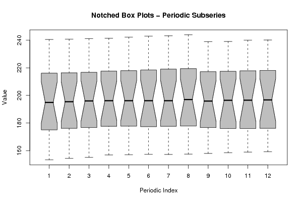
Figures (Output of Computation) | |||||||||||||||||||||
Input Parameters & R Code | |||||||||||||||||||||
| Parameters (Session): | |||||||||||||||||||||
| par1 = 12 ; | |||||||||||||||||||||
| Parameters (R input): | |||||||||||||||||||||
| par1 = 12 ; par2 = ; par3 = ; par4 = ; par5 = ; par6 = ; par7 = ; par8 = ; par9 = ; par10 = ; par11 = ; par12 = ; par13 = ; par14 = ; par15 = ; par16 = ; par17 = ; par18 = ; par19 = ; par20 = ; | |||||||||||||||||||||
| R code (references can be found in the software module): | |||||||||||||||||||||
par1 <- as.numeric(par1) | |||||||||||||||||||||