Free Statistics
of Irreproducible Research!
Description of Statistical Computation | |||||||||||||||||||||||||||||||||||||||||||||
|---|---|---|---|---|---|---|---|---|---|---|---|---|---|---|---|---|---|---|---|---|---|---|---|---|---|---|---|---|---|---|---|---|---|---|---|---|---|---|---|---|---|---|---|---|---|
| Author's title | |||||||||||||||||||||||||||||||||||||||||||||
| Author | *The author of this computation has been verified* | ||||||||||||||||||||||||||||||||||||||||||||
| R Software Module | rwasp_boxcoxlin.wasp | ||||||||||||||||||||||||||||||||||||||||||||
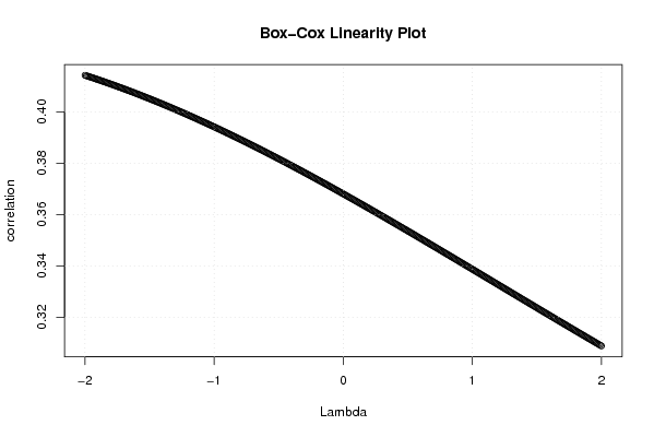
| Title produced by software | Box-Cox Linearity Plot | ||||||||||||||||||||||||||||||||||||||||||||
| Date of computation | Wed, 11 Nov 2009 03:22:53 -0700 | ||||||||||||||||||||||||||||||||||||||||||||
| Cite this page as follows | Statistical Computations at FreeStatistics.org, Office for Research Development and Education, URL https://freestatistics.org/blog/index.php?v=date/2009/Nov/11/t12579350970nv7lqw473uh79v.htm/, Retrieved Wed, 24 Apr 2024 21:36:07 +0000 | ||||||||||||||||||||||||||||||||||||||||||||
| Statistical Computations at FreeStatistics.org, Office for Research Development and Education, URL https://freestatistics.org/blog/index.php?pk=55463, Retrieved Wed, 24 Apr 2024 21:36:07 +0000 | |||||||||||||||||||||||||||||||||||||||||||||
| QR Codes: | |||||||||||||||||||||||||||||||||||||||||||||
|
| |||||||||||||||||||||||||||||||||||||||||||||
| Original text written by user: | |||||||||||||||||||||||||||||||||||||||||||||
| IsPrivate? | No (this computation is public) | ||||||||||||||||||||||||||||||||||||||||||||
| User-defined keywords | |||||||||||||||||||||||||||||||||||||||||||||
| Estimated Impact | 189 | ||||||||||||||||||||||||||||||||||||||||||||
Tree of Dependent Computations | |||||||||||||||||||||||||||||||||||||||||||||
| Family? (F = Feedback message, R = changed R code, M = changed R Module, P = changed Parameters, D = changed Data) | |||||||||||||||||||||||||||||||||||||||||||||
| - [Box-Cox Linearity Plot] [3/11/2009] [2009-11-02 21:47:57] [b98453cac15ba1066b407e146608df68] - D [Box-Cox Linearity Plot] [WS6 box cox] [2009-11-06 12:23:28] [8b1aef4e7013bd33fbc2a5833375c5f5] - [Box-Cox Linearity Plot] [] [2009-11-11 10:22:53] [2a6f24d4847085573f343c759dfbabef] [Current] | |||||||||||||||||||||||||||||||||||||||||||||
| Feedback Forum | |||||||||||||||||||||||||||||||||||||||||||||
Post a new message | |||||||||||||||||||||||||||||||||||||||||||||
Dataset | |||||||||||||||||||||||||||||||||||||||||||||
| Dataseries X: | |||||||||||||||||||||||||||||||||||||||||||||
100.00 100.00 97.56 95.12 92.68 92.68 97.56 107.32 112.20 112.20 112.20 114.63 117.07 117.07 114.63 114.63 114.63 112.20 121.95 131.71 134.15 136.59 136.59 141.46 146.34 148.78 148.78 146.34 146.34 148.78 158.54 173.17 180.49 180.49 182.93 185.37 190.24 190.24 187.80 185.37 182.93 178.05 185.37 195.12 195.12 192.68 190.24 187.80 190.24 187.80 182.93 178.05 173.17 170.73 178.05 190.24 192.68 192.68 190.24 190.24 192.68 190.24 185.37 180.49 175.61 168.29 173.17 182.93 185.37 180.49 178.05 175.61 178.05 175.61 173.17 170.73 168.29 165.85 175.61 185.37 187.80 185.37 182.93 182.93 185.37 185.37 185.37 182.93 178.05 175.61 180.49 195.12 200.00 195.12 187.80 187.80 190.24 190.24 187.80 182.93 178.05 173.17 173.17 175.61 165.85 160.98 156.10 156.10 158.54 153.66 143.90 134.15 126.83 119.51 131.71 141.46 139.02 136.59 134.15 131.71 131.71 131.71 134.15 141.46 139.02 131.71 136.59 141.46 151.22 165.85 163.41 163.41 156.10 153.66 153.66 156.10 153.66 146.34 153.66 153.66 160.98 182.93 190.24 192.68 190.24 185.37 182.93 185.37 182.93 178.05 185.37 182.93 185.37 192.68 192.68 197.56 200.00 195.12 182.93 165.85 158.54 160.98 185.37 195.12 197.56 187.80 182.93 185.37 190.24 190.24 190.24 182.93 182.93 173.17 182.93 182.93 185.37 187.80 187.80 192.68 197.56 200.00 200.00 200.00 192.68 178.05 168.29 160.98 163.41 168.29 170.73 173.17 175.61 173.17 168.29 170.73 165.85 156.10 163.41 160.98 156.10 153.66 151.22 158.54 165.85 165.85 156.10 148.78 141.46 148.78 175.61 178.05 168.29 148.78 141.46 151.22 173.17 187.80 192.68 187.80 180.49 182.93 195.12 197.56 | |||||||||||||||||||||||||||||||||||||||||||||
| Dataseries Y: | |||||||||||||||||||||||||||||||||||||||||||||
100.00 100.78 101.24 102.35 102.41 102.67 102.54 102.74 103.07 103.39 103.72 103.91 104.37 104.89 105.61 106.00 106.13 106.20 106.26 106.33 106.98 107.44 107.50 107.57 107.63 108.15 108.35 109.07 109.39 109.78 109.98 110.18 110.31 110.57 110.63 110.70 110.76 111.15 111.48 112.13 112.13 112.20 112.20 112.46 112.85 113.31 113.37 113.37 113.44 113.89 114.16 114.74 114.81 114.22 114.55 114.74 115.26 114.87 114.87 114.94 115.00 115.98 116.44 117.03 117.09 117.16 117.22 117.22 117.29 117.35 117.55 117.68 117.68 118.26 118.66 119.05 119.18 119.44 119.77 119.83 119.90 119.96 120.09 120.29 120.35 121.27 121.72 122.37 122.50 122.57 122.64 122.83 122.90 122.96 122.96 123.03 123.03 123.55 123.94 125.18 125.57 125.90 126.22 126.48 126.68 127.14 127.14 127.14 127.14 127.53 127.85 127.98 127.98 127.98 127.98 128.51 128.96 129.16 129.29 129.48 129.55 130.14 130.46 131.31 131.90 132.35 132.75 132.75 133.07 133.14 133.27 133.40 133.59 133.79 134.18 134.70 134.96 135.09 135.55 135.68 136.01 136.07 136.33 136.40 136.79 136.86 136.92 136.99 137.51 137.90 138.10 138.29 138.42 138.55 138.88 139.20 139.40 139.60 139.79 140.12 140.25 140.83 141.16 141.49 141.68 141.88 142.14 142.27 142.60 142.79 143.05 143.77 144.10 144.16 144.68 144.81 144.94 145.14 145.40 145.53 145.73 146.12 146.84 147.10 147.36 147.62 147.75 148.08 148.27 148.60 148.79 148.99 149.05 149.25 149.38 149.45 149.58 149.77 149.97 150.03 150.16 150.55 150.68 151.14 151.27 151.99 153.36 153.95 154.53 154.66 154.92 155.38 155.84 155.97 156.56 156.69 156.88 157.01 157.27 157.47 157.99 158.45 158.64 159.10 | |||||||||||||||||||||||||||||||||||||||||||||
Tables (Output of Computation) | |||||||||||||||||||||||||||||||||||||||||||||
| |||||||||||||||||||||||||||||||||||||||||||||
Figures (Output of Computation) | |||||||||||||||||||||||||||||||||||||||||||||
Input Parameters & R Code | |||||||||||||||||||||||||||||||||||||||||||||
| Parameters (Session): | |||||||||||||||||||||||||||||||||||||||||||||
| Parameters (R input): | |||||||||||||||||||||||||||||||||||||||||||||
| par1 = ; par2 = ; par3 = ; par4 = ; par5 = ; par6 = ; par7 = ; par8 = ; par9 = ; par10 = ; par11 = ; par12 = ; par13 = ; par14 = ; par15 = ; par16 = ; par17 = ; par18 = ; par19 = ; par20 = ; | |||||||||||||||||||||||||||||||||||||||||||||
| R code (references can be found in the software module): | |||||||||||||||||||||||||||||||||||||||||||||
n <- length(x) | |||||||||||||||||||||||||||||||||||||||||||||