Free Statistics
of Irreproducible Research!
Description of Statistical Computation | |||||||||||||||||||||||||||||||||||||||||||||||||||||||||||||||||
|---|---|---|---|---|---|---|---|---|---|---|---|---|---|---|---|---|---|---|---|---|---|---|---|---|---|---|---|---|---|---|---|---|---|---|---|---|---|---|---|---|---|---|---|---|---|---|---|---|---|---|---|---|---|---|---|---|---|---|---|---|---|---|---|---|---|
| Author's title | |||||||||||||||||||||||||||||||||||||||||||||||||||||||||||||||||
| Author | *The author of this computation has been verified* | ||||||||||||||||||||||||||||||||||||||||||||||||||||||||||||||||
| R Software Module | rwasp_edabi.wasp | ||||||||||||||||||||||||||||||||||||||||||||||||||||||||||||||||
| Title produced by software | Bivariate Explorative Data Analysis | ||||||||||||||||||||||||||||||||||||||||||||||||||||||||||||||||
| Date of computation | Tue, 10 Nov 2009 10:19:37 -0700 | ||||||||||||||||||||||||||||||||||||||||||||||||||||||||||||||||
| Cite this page as follows | Statistical Computations at FreeStatistics.org, Office for Research Development and Education, URL https://freestatistics.org/blog/index.php?v=date/2009/Nov/10/t1257873682cbygjes8mzhzvml.htm/, Retrieved Mon, 06 May 2024 04:18:24 +0000 | ||||||||||||||||||||||||||||||||||||||||||||||||||||||||||||||||
| Statistical Computations at FreeStatistics.org, Office for Research Development and Education, URL https://freestatistics.org/blog/index.php?pk=55320, Retrieved Mon, 06 May 2024 04:18:24 +0000 | |||||||||||||||||||||||||||||||||||||||||||||||||||||||||||||||||
| QR Codes: | |||||||||||||||||||||||||||||||||||||||||||||||||||||||||||||||||
|
| |||||||||||||||||||||||||||||||||||||||||||||||||||||||||||||||||
| Original text written by user: | |||||||||||||||||||||||||||||||||||||||||||||||||||||||||||||||||
| IsPrivate? | No (this computation is public) | ||||||||||||||||||||||||||||||||||||||||||||||||||||||||||||||||
| User-defined keywords | |||||||||||||||||||||||||||||||||||||||||||||||||||||||||||||||||
| Estimated Impact | 205 | ||||||||||||||||||||||||||||||||||||||||||||||||||||||||||||||||
Tree of Dependent Computations | |||||||||||||||||||||||||||||||||||||||||||||||||||||||||||||||||
| Family? (F = Feedback message, R = changed R code, M = changed R Module, P = changed Parameters, D = changed Data) | |||||||||||||||||||||||||||||||||||||||||||||||||||||||||||||||||
| - [Box-Cox Linearity Plot] [3/11/2009] [2009-11-02 21:47:57] [b98453cac15ba1066b407e146608df68] - RMPD [Bivariate Explorative Data Analysis] [] [2009-11-10 17:19:37] [6dfcce621b31349cab7f0d189e6f8a9d] [Current] - R PD [Bivariate Explorative Data Analysis] [] [2009-11-15 11:49:49] [f57b281e621ed7dff28b90886f5aa97c] - R PD [Bivariate Explorative Data Analysis] [] [2009-11-15 12:09:42] [f57b281e621ed7dff28b90886f5aa97c] - RMPD [Mean Plot] [] [2009-11-15 12:30:44] [f57b281e621ed7dff28b90886f5aa97c] - RMPD [Standard Deviation Plot] [] [2009-11-15 12:39:07] [f57b281e621ed7dff28b90886f5aa97c] - RMPD [Back to Back Histogram] [] [2009-11-15 12:49:53] [f57b281e621ed7dff28b90886f5aa97c] - PD [Bivariate Explorative Data Analysis] [Paper] [2010-12-26 09:33:15] [24bb5b06bd1854f48aebec8f44957ed0] | |||||||||||||||||||||||||||||||||||||||||||||||||||||||||||||||||
| Feedback Forum | |||||||||||||||||||||||||||||||||||||||||||||||||||||||||||||||||
Post a new message | |||||||||||||||||||||||||||||||||||||||||||||||||||||||||||||||||
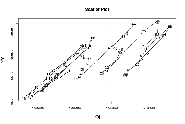
Dataset | |||||||||||||||||||||||||||||||||||||||||||||||||||||||||||||||||
| Dataseries X: | |||||||||||||||||||||||||||||||||||||||||||||||||||||||||||||||||
492865 480961 461935 456608 441977 439148 488180 520564 501492 485025 464196 460170 467037 460070 447988 442867 436087 431328 484015 509673 512927 502831 470984 471067 476049 474605 470439 461251 454724 455626 516847 525192 522975 518585 509239 512238 519164 517009 509933 509127 500857 506971 569323 579714 577992 565464 547344 554788 562325 560854 555332 543599 536662 542722 593530 610763 612613 611324 594167 595454 590865 589379 584428 573100 567456 569028 620735 628884 628232 612117 595404 597141 | |||||||||||||||||||||||||||||||||||||||||||||||||||||||||||||||||
| Dataseries Y: | |||||||||||||||||||||||||||||||||||||||||||||||||||||||||||||||||
116222 110924 103753 99983 93302 91496 119321 139261 133739 123913 113438 109416 109406 105645 101328 97686 93093 91382 122257 139183 139887 131822 116805 113706 113012 110452 107005 102841 98173 98181 137277 147579 146571 138920 130340 128140 127059 122860 117702 113537 108366 111078 150739 159129 157928 147768 137507 136919 136151 133001 125554 119647 114158 116193 152803 161761 160942 149470 139208 134588 130322 126611 122401 117352 112135 112879 148729 157230 157221 146681 136524 132111 | |||||||||||||||||||||||||||||||||||||||||||||||||||||||||||||||||
Tables (Output of Computation) | |||||||||||||||||||||||||||||||||||||||||||||||||||||||||||||||||
| |||||||||||||||||||||||||||||||||||||||||||||||||||||||||||||||||
Figures (Output of Computation) | |||||||||||||||||||||||||||||||||||||||||||||||||||||||||||||||||
Input Parameters & R Code | |||||||||||||||||||||||||||||||||||||||||||||||||||||||||||||||||
| Parameters (Session): | |||||||||||||||||||||||||||||||||||||||||||||||||||||||||||||||||
| par1 = red ; par2 = blue ; par3 = TRUE ; par4 = iptot ; par5 = ipkl ; | |||||||||||||||||||||||||||||||||||||||||||||||||||||||||||||||||
| Parameters (R input): | |||||||||||||||||||||||||||||||||||||||||||||||||||||||||||||||||
| par1 = 0 ; par2 = 36 ; | |||||||||||||||||||||||||||||||||||||||||||||||||||||||||||||||||
| R code (references can be found in the software module): | |||||||||||||||||||||||||||||||||||||||||||||||||||||||||||||||||
par1 <- as.numeric(par1) | |||||||||||||||||||||||||||||||||||||||||||||||||||||||||||||||||