Repository of Reproducible Computations

Free Statistics

of Irreproducible Research!

Author's title

Author

*The author of this computation has been verified*

R Software Module

rwasp_boxcoxlin.wasp

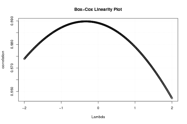
Title produced by software

Box-Cox Linearity Plot

Date of computation

Tue, 10 Nov 2009 04:13:46 -0700

Cite this page as follows

Statistical Computations at FreeStatistics.org, Office for Research Development and Education, URL https://freestatistics.org/blog/index.php?v=date/2009/Nov/10/t12578516609reo9ieoqh0kes9.htm/, Retrieved Mon, 06 May 2024 02:43:39 +0000

Statistical Computations at FreeStatistics.org, Office for Research Development and Education, URL https://freestatistics.org/blog/index.php?pk=55176, Retrieved Mon, 06 May 2024 02:43:39 +0000

QR Codes:

Paste this QR Code to cite your computation.

Original text written by user:

IsPrivate?

No (this computation is public)

User-defined keywords

Estimated Impact

165

Family? (F = Feedback message, R = changed R code, M = changed R Module, P = changed Parameters, D = changed Data)

-     [Box-Cox Linearity Plot] [3/11/2009] [2009-11-02 21:47:57] [b98453cac15ba1066b407e146608df68]
- R  D    [Box-Cox Linearity Plot] [] [2009-11-10 11:13:46] [2795ec65528c1a16d9df20713e7edc71] [Current]

Feedback Forum

Post a new message

Dataseries X:

Download CSV

Histogram

Boxplots

100
108.1560276
114.0150276
102.1880309
110.3672031
96.8602511
94.1944583
99.51621961
94.06333487
97.5541476
78.15062422
81.2434643
92.36262465
96.06324371
114.0523777
110.6616666
104.9171949
90.00187193
95.7008067
86.02741157
84.85287668
100.04328
80.91713823
74.06539709
77.30281369
97.23043249
90.75515676
100.5614455
92.01293267
99.24012138
105.8672755
90.9920463
93.30624423
91.17419413
77.33295039
91.1277721
85.01249943
83.90390242
104.8626302
110.9039108
95.43714373
111.6238727
108.8925403
96.17511682
101.9740205
99.11953031
86.78158147
118.4195003
118.7441447
106.5296192
134.7772694
104.6778714
105.2954304
139.4139849
103.6060491
99.78182974
103.4610301
120.0594945
96.71377168
107.1308929
105.3608372
111.6942359
132.0519998
126.8037879
154.4824253
141.5570984
109.9506882
127.904198
133.0888617
120.0796299
117.5557142
143.0362309
159.982927
128.5991124
149.7373327
126.8169313
140.9639674
137.6691981
117.9402337
122.3095247
127.7804207
136.1677176
116.2405856
123.1576893
116.3400234
108.6119282
125.8982264
112.8003105
107.5182447
135.0955413
115.5096488
115.8640759
104.5883906
163.7213386
113.4482275
98.0428844
116.7868521
126.5330444
113.0336597
124.3392163
109.8298759
124.4434777
111.5039454
102.0350019
116.8726598
112.2073122
101.1513902
124.4255108

Dataseries Y:

Download CSV

Histogram

100
211,3043478
333,9130435
187,826087
254,7826087
121,7391304
113,9130435
140,8695652
142,6086957
173,9130435
121,7391304
113,9130435
115,6521739
155,6521739
256,5217391
217,3913043
230,4347826
171,3043478
155,6521739
133,0434783
140,8695652
169,5652174
183,4782609
173,9130435
176,5217391
176,5217391
306,9565217
247,826087
171,3043478
140,8695652
171,3043478
153,0434783
184,3478261
236,5217391
177,3913043
164,3478261
208,6956522
211,3043478
403,4782609
328,6956522
261,7391304
254,7826087
277,3913043
282,6086957
357,3913043
284,3478261
183,4782609
186,0869565
179,1304348
175,6521739
317,3913043
375,6521739
277,3913043
313,9130435
203,4782609
199,1304348
240,8695652
238,2608696
258,2608696
335,6521739
302,6086957
373,9130435
570,4347826
382,6086957
307,826087
435,6521739
306,0869565
250,4347826
350,4347826
426,0869565
477,3913043
437,3913043
334,7826087
305,2173913
571,3043478
523,4782609
426,9565217
360,8695652
267,826087
254,7826087
357,3913043
348,6956522
259,1304348
290,4347826
329,5652174
304,3478261
566,9565217
409,5652174
345,2173913
445,2173913
315,6521739
270,4347826
306,0869565
326,9565217
313,0434783
300
360
334,7826087
384,3478261
531,3043478
325,2173913
399,1304348
365,2173913
216,5217391
333,9130435
348,6956522
180,8695652
292,173913

Summary of computational transaction
Raw Input	view raw input (R code)
Raw Output	view raw output of R engine
Computing time	2 seconds
R Server	'Gwilym Jenkins' @ 72.249.127.135

\begin{tabular}{lllllllll}
\hline
Summary of computational transaction \tabularnewline
Raw Input & view raw input (R code)  \tabularnewline
Raw Output & view raw output of R engine  \tabularnewline
Computing time & 2 seconds \tabularnewline
R Server & 'Gwilym Jenkins' @ 72.249.127.135 \tabularnewline
\hline
\end{tabular}
%Source: https://freestatistics.org/blog/index.php?pk=55176&T=0

[TABLE]
[ROW][C]Summary of computational transaction[/C][/ROW]
[ROW][C]Raw Input[/C][C]view raw input (R code) [/C][/ROW]
[ROW][C]Raw Output[/C][C]view raw output of R engine [/C][/ROW]
[ROW][C]Computing time[/C][C]2 seconds[/C][/ROW]
[ROW][C]R Server[/C][C]'Gwilym Jenkins' @ 72.249.127.135[/C][/ROW]
[/TABLE]
Source: https://freestatistics.org/blog/index.php?pk=55176&T=0

Globally Unique Identifier (entire table): ba.freestatistics.org/blog/index.php?pk=55176&T=0

As an alternative you can also use a QR Code:

The GUIDs for individual cells are displayed in the table below:

Summary of computational transaction
Raw Input	view raw input (R code)
Raw Output	view raw output of R engine
Computing time	2 seconds
R Server	'Gwilym Jenkins' @ 72.249.127.135

Box-Cox Linearity Plot
# observations x	108
maximum correlation	0.68982084589958
optimal lambda(x)	-0.33
Residual SD (orginial)	79.4267959035408
Residual SD (transformed)	78.3257718455003

\begin{tabular}{lllllllll}
\hline
Box-Cox Linearity Plot \tabularnewline
# observations x & 108 \tabularnewline
maximum correlation & 0.68982084589958 \tabularnewline
optimal lambda(x) & -0.33 \tabularnewline
Residual SD (orginial) & 79.4267959035408 \tabularnewline
Residual SD (transformed) & 78.3257718455003 \tabularnewline
\hline
\end{tabular}
%Source: https://freestatistics.org/blog/index.php?pk=55176&T=1

[TABLE]
[ROW][C]Box-Cox Linearity Plot[/C][/ROW]
[ROW][C]# observations x[/C][C]108[/C][/ROW]
[ROW][C]maximum correlation[/C][C]0.68982084589958[/C][/ROW]
[ROW][C]optimal lambda(x)[/C][C]-0.33[/C][/ROW]
[ROW][C]Residual SD (orginial)[/C][C]79.4267959035408[/C][/ROW]
[ROW][C]Residual SD (transformed)[/C][C]78.3257718455003[/C][/ROW]
[/TABLE]
Source: https://freestatistics.org/blog/index.php?pk=55176&T=1

Globally Unique Identifier (entire table): ba.freestatistics.org/blog/index.php?pk=55176&T=1

As an alternative you can also use a QR Code:

The GUIDs for individual cells are displayed in the table below:

Box-Cox Linearity Plot
# observations x	108
maximum correlation	0.68982084589958
optimal lambda(x)	-0.33
Residual SD (orginial)	79.4267959035408
Residual SD (transformed)	78.3257718455003

Figure 1

PNG link

Postscript link

PDF link

Figure 2

PNG link

Postscript link

PDF link

Figure 3

PNG link

Postscript link

PDF link

Parameters (Session):

Parameters (R input):

R code (references can be found in the software module):

n <- length(x)
c <- array(NA,dim=c(401))
l <- array(NA,dim=c(401))
mx <- 0
mxli <- -999
for (i in 1:401)
{
l[i] <- (i-201)/100
if (l[i] != 0)
{
x1 <- (x^l[i] - 1) / l[i]
} else {
x1 <- log(x)
}
c[i] <- cor(x1,y)
if (mx < abs(c[i]))
{
mx <- abs(c[i])
mxli <- l[i]
}
}
c
mx
mxli
if (mxli != 0)
{
x1 <- (x^mxli - 1) / mxli
} else {
x1 <- log(x)
}
r<-lm(y~x)
se <- sqrt(var(r$residuals))
r1 <- lm(y~x1)
se1 <- sqrt(var(r1$residuals))
bitmap(file='test1.png')
plot(l,c,main='Box-Cox Linearity Plot',xlab='Lambda',ylab='correlation')
grid()
dev.off()
bitmap(file='test2.png')
plot(x,y,main='Linear Fit of Original Data',xlab='x',ylab='y')
abline(r)
grid()
mtext(paste('Residual Standard Deviation = ',se))
dev.off()
bitmap(file='test3.png')
plot(x1,y,main='Linear Fit of Transformed Data',xlab='x',ylab='y')
abline(r1)
grid()
mtext(paste('Residual Standard Deviation = ',se1))
dev.off()
load(file='createtable')
a<-table.start()
a<-table.row.start(a)
a<-table.element(a,'Box-Cox Linearity Plot',2,TRUE)
a<-table.row.end(a)
a<-table.row.start(a)
a<-table.element(a,'# observations x',header=TRUE)
a<-table.element(a,n)
a<-table.row.end(a)
a<-table.row.start(a)
a<-table.element(a,'maximum correlation',header=TRUE)
a<-table.element(a,mx)
a<-table.row.end(a)
a<-table.row.start(a)
a<-table.element(a,'optimal lambda(x)',header=TRUE)
a<-table.element(a,mxli)
a<-table.row.end(a)
a<-table.row.start(a)
a<-table.element(a,'Residual SD (orginial)',header=TRUE)
a<-table.element(a,se)
a<-table.row.end(a)
a<-table.row.start(a)
a<-table.element(a,'Residual SD (transformed)',header=TRUE)
a<-table.element(a,se1)
a<-table.row.end(a)
a<-table.end(a)
table.save(a,file='mytable.tab')

Free Statistics

Description of Statistical Computation

Tree of Dependent Computations

Dataset

Tables (Output of Computation)

Figures (Output of Computation)

Input Parameters & R Code