Free Statistics
of Irreproducible Research!
Description of Statistical Computation | |||||||||||||||||||||
|---|---|---|---|---|---|---|---|---|---|---|---|---|---|---|---|---|---|---|---|---|---|
| Author's title | |||||||||||||||||||||
| Author | *The author of this computation has been verified* | ||||||||||||||||||||
| R Software Module | rwasp_sdplot.wasp | ||||||||||||||||||||
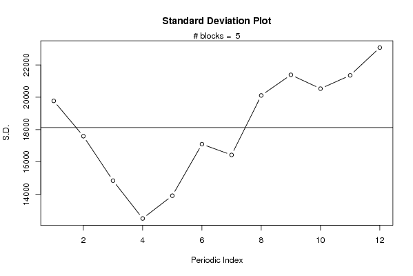
| Title produced by software | Standard Deviation Plot | ||||||||||||||||||||
| Date of computation | Mon, 09 Nov 2009 17:37:57 -0700 | ||||||||||||||||||||
| Cite this page as follows | Statistical Computations at FreeStatistics.org, Office for Research Development and Education, URL https://freestatistics.org/blog/index.php?v=date/2009/Nov/10/t12578135090ufsajezspp8fup.htm/, Retrieved Mon, 06 May 2024 05:14:18 +0000 | ||||||||||||||||||||
| Statistical Computations at FreeStatistics.org, Office for Research Development and Education, URL https://freestatistics.org/blog/index.php?pk=55110, Retrieved Mon, 06 May 2024 05:14:18 +0000 | |||||||||||||||||||||
| QR Codes: | |||||||||||||||||||||
|
| |||||||||||||||||||||
| Original text written by user: | |||||||||||||||||||||
| IsPrivate? | No (this computation is public) | ||||||||||||||||||||
| User-defined keywords | |||||||||||||||||||||
| Estimated Impact | 208 | ||||||||||||||||||||
Tree of Dependent Computations | |||||||||||||||||||||
| Family? (F = Feedback message, R = changed R code, M = changed R Module, P = changed Parameters, D = changed Data) | |||||||||||||||||||||
| - [Standard Deviation Plot] [3/11/2009] [2009-11-02 22:09:58] [b98453cac15ba1066b407e146608df68] - R D [Standard Deviation Plot] [WorkShop6 (SHW)] [2009-11-10 00:37:57] [d41d8cd98f00b204e9800998ecf8427e] [Current] - PD [Standard Deviation Plot] [Ws6, Part 9.3] [2009-11-12 15:25:50] [aba88da643e3763d32ff92bd8f92a385] - D [Standard Deviation Plot] [Workshop 6] [2009-11-12 15:25:50] [b6394cb5c2dcec6d17418d3cdf42d699] - D [Standard Deviation Plot] [workshop 6 standa...] [2009-11-12 15:25:57] [af8eb90b4bf1bcfcc4325c143dbee260] | |||||||||||||||||||||
| Feedback Forum | |||||||||||||||||||||
Post a new message | |||||||||||||||||||||
Dataset | |||||||||||||||||||||
| Dataseries X: | |||||||||||||||||||||
282965 276610 277838 277051 277026 274960 270073 267063 264916 287182 291109 292223 288109 281400 282579 280113 280331 276759 275139 274275 271234 289725 290649 292223 278429 269749 265784 268957 264099 255121 253276 245980 235295 258479 260916 254586 250566 243345 247028 248464 244962 237003 237008 225477 226762 247857 248256 246892 245021 246186 255688 264242 268270 272969 273886 267353 271916 292633 295804 293222 | |||||||||||||||||||||
Tables (Output of Computation) | |||||||||||||||||||||
| |||||||||||||||||||||
Figures (Output of Computation) | |||||||||||||||||||||
Input Parameters & R Code | |||||||||||||||||||||
| Parameters (Session): | |||||||||||||||||||||
| Parameters (R input): | |||||||||||||||||||||
| par1 = 12 ; | |||||||||||||||||||||
| R code (references can be found in the software module): | |||||||||||||||||||||
par1 <- as.numeric(par1) | |||||||||||||||||||||