Repository of Reproducible Computations

Free Statistics

of Irreproducible Research!

Author's title

Author

*The author of this computation has been verified*

R Software Module

rwasp_pairs.wasp

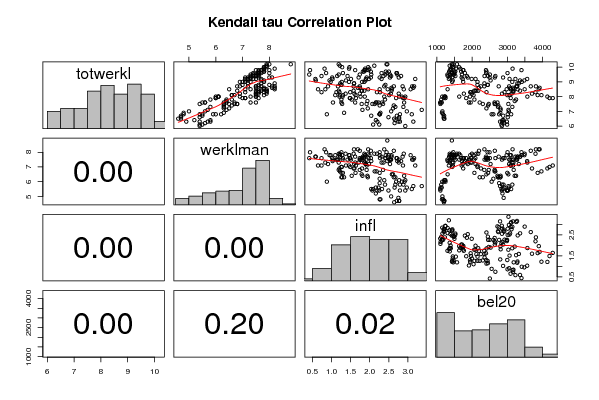
Title produced by software

Kendall tau Correlation Matrix

Date of computation

Mon, 09 Nov 2009 11:36:43 -0700

Cite this page as follows

Statistical Computations at FreeStatistics.org, Office for Research Development and Education, URL https://freestatistics.org/blog/index.php?v=date/2009/Nov/09/t1257791835p0qzfngyutjmdss.htm/, Retrieved Sat, 20 Apr 2024 09:30:45 +0000

Statistical Computations at FreeStatistics.org, Office for Research Development and Education, URL https://freestatistics.org/blog/index.php?pk=54913, Retrieved Sat, 20 Apr 2024 09:30:45 +0000

QR Codes:

Paste this QR Code to cite your computation.

Original text written by user:

IsPrivate?

No (this computation is public)

User-defined keywords

Estimated Impact

200

Family? (F = Feedback message, R = changed R code, M = changed R Module, P = changed Parameters, D = changed Data)

-     [Kendall tau Correlation Matrix] [3/11/2009] [2009-11-02 21:25:00] [b98453cac15ba1066b407e146608df68]
- R  D    [Kendall tau Correlation Matrix] [workshop 6] [2009-11-09 18:36:43] [e81f30a5c3daacfe71a556c99a478849] [Current]
-    D      [Kendall tau Correlation Matrix] [paper] [2009-12-18 23:23:51] [3d8acb8ffdb376c5fec19e610f8198c2] 

Feedback Forum

Post a new message

Dataseries X:

Download CSV

Histogram

Boxplots

6.9	4.8	2.28	1145.11
6.8	4.8	2.26	1176.86
6.7	4.7	2.71	1206.41
6.6	4.7	2.77	1192.72
6.5	4.7	2.77	1214.82
6.5	4.6	2.64	1199.07
7.0	5.0	2.56	1157.47
7.5	5.4	2.07	1100.10
7.6	5.5	2.32	1095.63
7.6	5.6	2.16	1105.63
7.6	5.6	2.23	1137.79
7.8	5.8	2.40	1124.72
8.0	6.0	2.84	1152.60
8.0	6.1	2.77	1211.85
8.0	6.1	2.93	1239.62
7.9	6.0	2.91	1244.13
7.9	6.0	2.69	1198.42
8.0	6.1	2.38	1227.99
8.5	6.5	2.58	1304.92
9.2	7.1	3.19	1340.26
9.4	7.4	2.82	1307.32
9.5	7.4	2.72	1356.51
9.5	7.5	2.53	1383.29
9.6	7.6	2.70	1437.87
9.7	7.8	2.42	1494.56
9.7	7.8	2.50	1521.42
9.6	7.7	2.31	1498.76
9.5	7.6	2.41	1488.75
9.4	7.5	2.56	1524.62
9.3	7.3	2.76	1439.27
9.6	7.6	2.71	1423.11
10.2	8.0	2.44	1466.85
10.2	8.8	2.46	1425.83
10.1	7.9	2.12	1363.45
9.9	7.8	1.99	1389.18
9.8	7.7	1.86	1395.89
9.8	7.8	1.88	1368.43
9.7	7.7	1.82	1349.03
9.5	7.5	1.74	1299.88
9.3	7.3	1.71	1365.41
9.1	7.1	1.38	1451.04
9.0	7.0	1.27	1433.75
9.5	7.3	1.19	1464.65
10.0	7.8	1.28	1475.57
10.2	7.9	1.19	1571.16
10.1	7.9	1.22	1429.12
10.0	7.8	1.47	1452.46
9.9	7.8	1.46	1538.09
10.0	7.9	1.96	1631.59
9.9	7.8	1.88	1665.50
9.7	7.6	2.03	1690.60
9.5	7.4	2.04	1711.74
9.2	7.2	1.90	1734.10
9.0	6.9	1.80	1748.09
9.3	7.1	1.92	1703.45
9.8	7.5	1.92	1745.74
9.8	7.6	1.97	1751.01
9.6	7.4	2.46	1795.65
9.4	7.3	2.36	1852.13
9.3	7.2	2.53	1877.10
9.2	7.3	2.31	1989.31
9.2	7.2	1.98	2097.76
9.0	7.1	1.46	2154.87
8.8	7.0	1.26	2152.18
8.7	6.9	1.58	2250.27
8.7	6.8	1.74	2346.90
9.1	7.2	1.89	2525.56
9.7	7.6	1.85	2409.36
9.8	7.7	1.62	2394.36
9.6	7.6	1.30	2401.33
9.4	7.5	1.42	2354.32
9.4	7.5	1.15	2450.41
9.5	7.6	0.42	2504.67
9.4	7.6	0.74	2661.39
9.3	7.6	1.02	2880.40
9.2	7.5	1.51	3064.42
9.0	7.3	1.86	3141.12
8.9	7.2	1.59	3327.70
9.2	7.4	1.03	3564.95
9.8	8.0	0.44	3403.13
9.9	8.2	0.82	3149.90
9.6	8.0	0.86	3006.84
9.2	7.7	0.58	3230.66
9.1	7.7	0.59	3361.13
9.1	7.8	0.95	3484.74
9.0	7.8	0.98	3411.13
8.9	7.7	1.23	3288.18
8.7	7.5	1.17	3280.37
8.5	7.3	0.84	3173.95
8.3	7.1	0.74	3165.26
8.5	7.1	0.65	3092.71
8.7	7.2	0.91	3053.05
8.4	6.8	1.19	3181.96
8.1	6.6	1.30	2999.93
7.8	6.4	1.53	3249.57
7.7	6.4	1.94	3210.52
7.5	6.5	1.79	3030.29
7.2	6.3	1.95	2803.47
6.8	5.9	2.26	2767.63
6.7	5.5	2.04	2882.60
6.4	5.2	2.16	2863.36
6.3	4.9	2.75	2897.06
6.8	5.4	2.79	3012.61
7.3	5.8	2.88	3142.95
7.1	5.7	3.36	3032.93
7.0	5.6	2.97	3045.78
6.8	5.5	3.10	3110.52
6.6	5.4	2.49	3013.24
6.3	5.4	2.20	2987.10
6.1	5.4	2.25	2995.55
6.1	5.5	2.09	2833.18
6.3	5.8	2.79	2848.96
6.3	5.7	3.14	2794.83
6.0	5.4	2.93	2845.26
6.2	5.6	2.65	2915.02
6.4	5.8	2.67	2892.63
6.8	6.2	2.26	2604.42
7.5	6.8	2.35	2641.65
7.5	6.7	2.13	2659.81
7.6	6.7	2.18	2638.53
7.6	6.4	2.90	2720.25
7.4	6.3	2.63	2745.88
7.3	6.3	2.67	2735.70
7.1	6.4	1.81	2811.70
6.9	6.3	1.33	2799.43
6.8	6.0	0.88	2555.28
7.5	6.3	1.28	2304.98
7.6	6.3	1.26	2214.95
7.8	6.6	1.26	2065.81
8.0	7.5	1.29	1940.49
8.1	7.8	1.10	2042.00
8.2	7.9	1.37	1995.37
8.3	7.8	1.21	1946.81
8.2	7.6	1.74	1765.90
8.0	7.5	1.76	1635.25
7.9	7.6	1.48	1833.42
7.6	7.5	1.04	1910.43
7.6	7.3	1.62	1959.67
8.3	7.6	1.49	1969.60
8.4	7.5	1.79	2061.41
8.4	7.6	1.80	2093.48
8.4	7.9	1.58	2120.88
8.4	7.9	1.86	2174.56
8.6	8.1	1.74	2196.72
8.9	8.2	1.59	2350.44
8.8	8.0	1.26	2440.25
8.3	7.5	1.13	2408.64
7.5	6.8	1.92	2472.81
7.2	6.5	2.61	2407.60
7.4	6.6	2.26	2454.62
8.8	7.6	2.41	2448.05
9.3	8.0	2.26	2497.84
9.3	8.1	2.03	2645.64
8.7	7.7	2.86	2756.76
8.2	7.5	2.55	2849.27
8.3	7.6	2.27	2921.44
8.5	7.8	2.26	2981.85
8.6	7.8	2.57	3080.58
8.5	7.8	3.07	3106.22
8.2	7.5	2.76	3119.31
8.1	7.5	2.51	3061.26
7.9	7.1	2.87	3097.31
8.6	7.5	3.14	3161.69
8.7	7.5	3.11	3257.16
8.7	7.6	3.16	3277.01
8.5	7.7	2.47	3295.32
8.4	7.7	2.57	3363.99
8.5	7.9	2.89	3494.17
8.7	8.1	2.63	3667.03
8.7	8.2	2.38	3813.06
8.6	8.2	1.69	3917.96
8.5	8.2	1.96	3895.51
8.3	7.9	2.19	3801.06
8.0	7.3	1.87	3570.12
8.2	6.9	1.6	3701.61
8.1	6.6	1.63	3862.27
8.1	6.7	1.22	3970.10
8.0	6.9	1.21	4138.52
7.9	7.0	1.49	4199.75
7.9	7.1	1.64	4290.89

Summary of computational transaction
Raw Input	view raw input (R code)
Raw Output	view raw output of R engine
Computing time	1 seconds
R Server	'Gwilym Jenkins' @ 72.249.127.135

\begin{tabular}{lllllllll}
\hline
Summary of computational transaction \tabularnewline
Raw Input & view raw input (R code)  \tabularnewline
Raw Output & view raw output of R engine  \tabularnewline
Computing time & 1 seconds \tabularnewline
R Server & 'Gwilym Jenkins' @ 72.249.127.135 \tabularnewline
\hline
\end{tabular}
%Source: https://freestatistics.org/blog/index.php?pk=54913&T=0

[TABLE]
[ROW][C]Summary of computational transaction[/C][/ROW]
[ROW][C]Raw Input[/C][C]view raw input (R code) [/C][/ROW]
[ROW][C]Raw Output[/C][C]view raw output of R engine [/C][/ROW]
[ROW][C]Computing time[/C][C]1 seconds[/C][/ROW]
[ROW][C]R Server[/C][C]'Gwilym Jenkins' @ 72.249.127.135[/C][/ROW]
[/TABLE]
Source: https://freestatistics.org/blog/index.php?pk=54913&T=0

Globally Unique Identifier (entire table): ba.freestatistics.org/blog/index.php?pk=54913&T=0

As an alternative you can also use a QR Code:

The GUIDs for individual cells are displayed in the table below:

Summary of computational transaction
Raw Input	view raw input (R code)
Raw Output	view raw output of R engine
Computing time	1 seconds
R Server	'Gwilym Jenkins' @ 72.249.127.135

Kendall tau rank correlations for all pairs of data series
pair	tau	p-value
tau( totwerkl , werklman )	0.598856841359808	0
tau( totwerkl , infl )	-0.196193610266963	0.000115102473078996
tau( totwerkl , bel20 )	-0.147186544830462	0.00374156474602443
tau( werklman , infl )	-0.218104045412738	2.11417624322091e-05
tau( werklman , bel20 )	0.0655870282497056	0.200024452173624
tau( infl , bel20 )	-0.121679915168396	0.0155179162239798

\begin{tabular}{lllllllll}
\hline
Kendall tau rank correlations for all pairs of data series \tabularnewline
pair & tau & p-value \tabularnewline
tau( totwerkl , werklman ) & 0.598856841359808 & 0 \tabularnewline
tau( totwerkl , infl ) & -0.196193610266963 & 0.000115102473078996 \tabularnewline
tau( totwerkl , bel20 ) & -0.147186544830462 & 0.00374156474602443 \tabularnewline
tau( werklman , infl ) & -0.218104045412738 & 2.11417624322091e-05 \tabularnewline
tau( werklman , bel20 ) & 0.0655870282497056 & 0.200024452173624 \tabularnewline
tau( infl , bel20 ) & -0.121679915168396 & 0.0155179162239798 \tabularnewline
\hline
\end{tabular}
%Source: https://freestatistics.org/blog/index.php?pk=54913&T=1

[TABLE]
[ROW][C]Kendall tau rank correlations for all pairs of data series[/C][/ROW]
[ROW][C]pair[/C][C]tau[/C][C]p-value[/C][/ROW]
[ROW][C]tau( totwerkl , werklman )[/C][C]0.598856841359808[/C][C]0[/C][/ROW]
[ROW][C]tau( totwerkl , infl )[/C][C]-0.196193610266963[/C][C]0.000115102473078996[/C][/ROW]
[ROW][C]tau( totwerkl , bel20 )[/C][C]-0.147186544830462[/C][C]0.00374156474602443[/C][/ROW]
[ROW][C]tau( werklman , infl )[/C][C]-0.218104045412738[/C][C]2.11417624322091e-05[/C][/ROW]
[ROW][C]tau( werklman , bel20 )[/C][C]0.0655870282497056[/C][C]0.200024452173624[/C][/ROW]
[ROW][C]tau( infl , bel20 )[/C][C]-0.121679915168396[/C][C]0.0155179162239798[/C][/ROW]
[/TABLE]
Source: https://freestatistics.org/blog/index.php?pk=54913&T=1

Globally Unique Identifier (entire table): ba.freestatistics.org/blog/index.php?pk=54913&T=1

As an alternative you can also use a QR Code:

The GUIDs for individual cells are displayed in the table below:

Kendall tau rank correlations for all pairs of data series
pair	tau	p-value
tau( totwerkl , werklman )	0.598856841359808	0
tau( totwerkl , infl )	-0.196193610266963	0.000115102473078996
tau( totwerkl , bel20 )	-0.147186544830462	0.00374156474602443
tau( werklman , infl )	-0.218104045412738	2.11417624322091e-05
tau( werklman , bel20 )	0.0655870282497056	0.200024452173624
tau( infl , bel20 )	-0.121679915168396	0.0155179162239798

Figure 1

PNG link

Postscript link

PDF link

Parameters (Session):

Parameters (R input):

R code (references can be found in the software module):

panel.tau <- function(x, y, digits=2, prefix='', cex.cor)
{
usr <- par('usr'); on.exit(par(usr))
par(usr = c(0, 1, 0, 1))
rr <- cor.test(x, y, method='kendall')
r <- round(rr$p.value,2)
txt <- format(c(r, 0.123456789), digits=digits)[1]
txt <- paste(prefix, txt, sep='')
if(missing(cex.cor)) cex <- 0.5/strwidth(txt)
text(0.5, 0.5, txt, cex = cex)
}
panel.hist <- function(x, ...)
{
usr <- par('usr'); on.exit(par(usr))
par(usr = c(usr[1:2], 0, 1.5) )
h <- hist(x, plot = FALSE)
breaks <- h$breaks; nB <- length(breaks)
y <- h$counts; y <- y/max(y)
rect(breaks[-nB], 0, breaks[-1], y, col='grey', ...)
}
bitmap(file='test1.png')
pairs(t(y),diag.panel=panel.hist, upper.panel=panel.smooth, lower.panel=panel.tau, main=main)
dev.off()
load(file='createtable')
a<-table.start()
a<-table.row.start(a)
a<-table.element(a,'Kendall tau rank correlations for all pairs of data series',3,TRUE)
a<-table.row.end(a)
a<-table.row.start(a)
a<-table.element(a,'pair',1,TRUE)
a<-table.element(a,'tau',1,TRUE)
a<-table.element(a,'p-value',1,TRUE)
a<-table.row.end(a)
n <- length(y[,1])
n
cor.test(y[1,],y[2,],method='kendall')
for (i in 1:(n-1))
{
for (j in (i+1):n)
{
a<-table.row.start(a)
dum <- paste('tau(',dimnames(t(x))[[2]][i])
dum <- paste(dum,',')
dum <- paste(dum,dimnames(t(x))[[2]][j])
dum <- paste(dum,')')
a<-table.element(a,dum,header=TRUE)
r <- cor.test(y[i,],y[j,],method='kendall')
a<-table.element(a,r$estimate)
a<-table.element(a,r$p.value)
a<-table.row.end(a)
}
}
a<-table.end(a)
table.save(a,file='mytable.tab')

Free Statistics

Description of Statistical Computation

Tree of Dependent Computations

Dataset

Tables (Output of Computation)

Figures (Output of Computation)

Input Parameters & R Code